Loading [Contrib]/a11y/accessibility-menu.js
Skip to main content
null
Findings
  • Menu
  • Articles
    • Energy Findings
    • Resilience Findings
    • Safety Findings
    • Transport Findings
    • Urban Findings
    • All
  • For Authors
  • Editorial Board
  • About
  • Blog
  • covid-19
  • search

RSS Feed

Enter the URL below into your favorite RSS reader.

http://localhost:54963/feed
Transport Findings
November 17, 2023 AEST

Intercomparison of Six National Empirical Models for PM2.5 Air Pollution in the Contiguous US

Matthew J. Bechle, Michelle L. Bell, Daniel L. Goldberg, Steve Hankey, Tianjun Lu, Albert A. Presto, Allen L. Robinson, Joel Schwartz, Liuhua Shi, Yang Zhang, Julian D. Marshall,
Land use regressionexposure assessmentair quality modelsempirical model comparisonpoint-based modelsgridded modelsair pollutionenvironmental findingsenvironmentparticulate matter
Copyright Logoccby-sa-4.0 • https://doi.org/10.32866/001c.89423
Photo by Jacek Dylag on Unsplash
Findings
Bechle, Matthew J., Michelle L. Bell, Daniel L. Goldberg, Steve Hankey, Tianjun Lu, Albert A. Presto, Allen L. Robinson, et al. 2023. “Intercomparison of Six National Empirical Models for PM2.5 Air Pollution in the Contiguous US.” Findings, November. https:/​/​doi.org/​10.32866/​001c.89423.
Save article as...▾
Download all (5)
  • Table 1. Summary of models and processing steps
    Download
  • Figure 1. Scatterplot matrix for year-2010 tract-level PM2.5.
    Download
  • Figure 2. Summary of pairwise Pearson correlation coefficients (top) and root mean square difference (bottom) for all locations, urban and rural locations, and NOAA climate regions.
    Download
  • Figure 3. Variability by concentration and location.
    Download
  • Supplemental Information
    Download

Sorry, something went wrong. Please try again.

If this problem reoccurs, please contact Scholastica Support

Error message:

undefined

View more stats

Abstract

Empirical models aim to predict spatial variability in concentrations of outdoor air pollution. For year-2010 concentrations of PM2.5 in the US, we intercompared six national-scale empirical models, each generated by a different research group. Despite differences in methods and independent variables for the models, we find a relatively high degree of agreement among model predictions (e.g., correlations of 0.84 to 0.92, RMSD (root-mean-square-difference; units: μg/m3) of 0.8 to 1.4, or on average ~12% of the average concentration; many best-fit lines are near the 1:1 line).

1. Questions

Our question is, how do concentration predictions from six annual-average ambient PM2.5 empirical models for the contiguous US compare with each other? We investigate this question at three spatial scales: nationally, regionally, and urban/rural. Our two hypotheses are that model predictions will be (1) relatively similar to each other, because the models all use (as the dependent variable) publicly-available data from regulatory monitoring stations, or (2) relatively dissimilar because models differ in their methods and independent variables.

2. Methods

2.1. Input data

We obtained year-2010 predicted fine particulate matter (PM2.5) concentrations for six empirical models (see Table 1) via data download or direct request from researchers. Three models are “point based” (concentrations predicted at specific spatial locations):

  1. CACES EPA-ACE: universal kriging with partial least squares data-reduction (PLS-UK) (Kim et al. 2020).

  2. EPA downscaler: Bayesian space-time “fuse” of monitoring data and 12 km CMAQ model outputs (US EPA 2022).

  3. MESA-Air models: space-time PLS with expectation-maximization to fill in missing observations (Keller et al. 2015).

The other three models are “gridded” (predictions are the spatial average within a grid-cell [e.g., a ~ 1 km2 area]):

  1. Harvard/MIT EPA-ACE: generalized additive model, integrating multiple machine-learning algorithms (Di et al. 2019a).

  2. SEARCH EPA-ACE: fusion of WRF-Chem, satellite data (MAIAC AOD), and a kriging of EPA monitor data (Goldberg et al. 2019).

  3. van Donkelaar et al. (2019): statistically “fuses” a chemical transport model (GEOS-Chem), satellite observations of aerosol optical depth, and ground-based observations using a geographically weighted regression.

Table 1
Table 1.Summary of models and processing steps

a CACES and EPA downscaler ozone modeled as 5-month (May-Sept) ozone season average of daily 8-hr max.
1. Kim et al. 2020.
2. US EPA 2017 and US EPA 2022.
3. Sampson et al. 2013.
4. Young et al. 2016.
5. Di et al. 2019a.
6. Di et al. 2019b.
7. Requia et al. 2020.
8. Goldberg et al. 2019.
9. van Donkelaar et al. 2019.

2.2. Processing of input data

We aligned spatiotemporal aspects of the models to be annual-average, by Census Tract (n ~ 74,000). For sub-annual (e.g., monthly) predictions, we calculated annual averages; for sub-tract predictions, we calculated Tract means; for gridded predictions, we converted to Census geographies by extracting values at block locations and then population weighting to the tract level.

One of the models (SEARCH model) is only available for the eastern half of the contiguous US (90° W longitude), which includes US cities as far west as Chicago. The other five models are available for the contiguous US.

2.3. Analysis

We conducted three pairwise comparisons of the model-predictions: (1) scatterplot matrices, (2) Pearson’s r, and (3) root mean square difference (RMSD) between predictions. We also generated boxplots showing distribution of predictions, and calculated the two values in each tract to indicate the range of model predictions: range (i.e., max minus min), and trimmed range (second-highest value minus second-lowest value).

We compare the individual model predictions against the median prediction of all models. The median measures central-tendency across models; absent further information, the median represents a “best estimate” or “ensemble forecast”. This study conducts model-model comparisons; it does not compare model predictions to monitoring or “gold-standard” data.

We conducted comparisons for (1) all locations, (2) urban vs. rural (urban defined as all tracts intersecting with Census urbanized areas, all remaining tracts are considered rural), (3) by region (using the 9 NOAA climate regions), and (4) stratified by population density (using the 2010 tract-level population density).

3. Findings

Predicted year-2010 PM2.5 concentrations range from ~2 to ~15 μg/m3. Pairwise scatterplots of model predictions (Figure 1) indicate a relatively high degree of agreement. The average Pearson correlation coefficient ("r") is 0.87 (range: 0.84 to 0.92), RMSD (units: μg/m3) is 1.1 on average (range: 0.8 to 1.4), and many best-fit lines are near the 1:1 line. The population average concentration of PM2.5 in 2010 was ~9.3 μg/m3 (mean), ~9.5 μg/m3 (median), so the RMSD (1.1 μg/m3) represents ~12% of the average concentration. Thus, nationally, the models agree well, supporting hypothesis #1, not #2.

Figure 1
Figure 1.Scatterplot matrix for year-2010 tract-level PM2.5.

Scatterplots in the upper right show pairwise tract-level predictions (µg/m3; n ~ 74,000 from each model except SEARCH). Grey dashed line shows 1:1 line, red solid line shows linear trendline. Corresponding boxes in the bottom left show Pearson’s correlation (r; unitless) and root mean squared difference (RMSD; µg/m3) between model predictions.

When comparing the models separately by geographic region (Figure 2), we see modest differences among models for most regions, and minor differences between urban/rural locations. Based on r, model-model agreement is slightly lower in the Midwest and South than in other regions. RMSDs indicate agreement is slightly lower in the West.

Figure 2
Figure 2.Summary of pairwise Pearson correlation coefficients (top) and root mean square difference (bottom) for all locations, urban and rural locations, and NOAA climate regions.

Horizontal bar shows the median, box shows the interquartile range, and vertical lines show max and min values among model comparisons. The six NOAA regions denoted with an asterisk (“*”) exclude SEARCH predictions as they were unavailable geographically. The results for those six regions reflect the n=10 pairwise comparisons of five models; results for the other regions (without an asterisk) reflect the n=15 pairwise comparisons of six models.

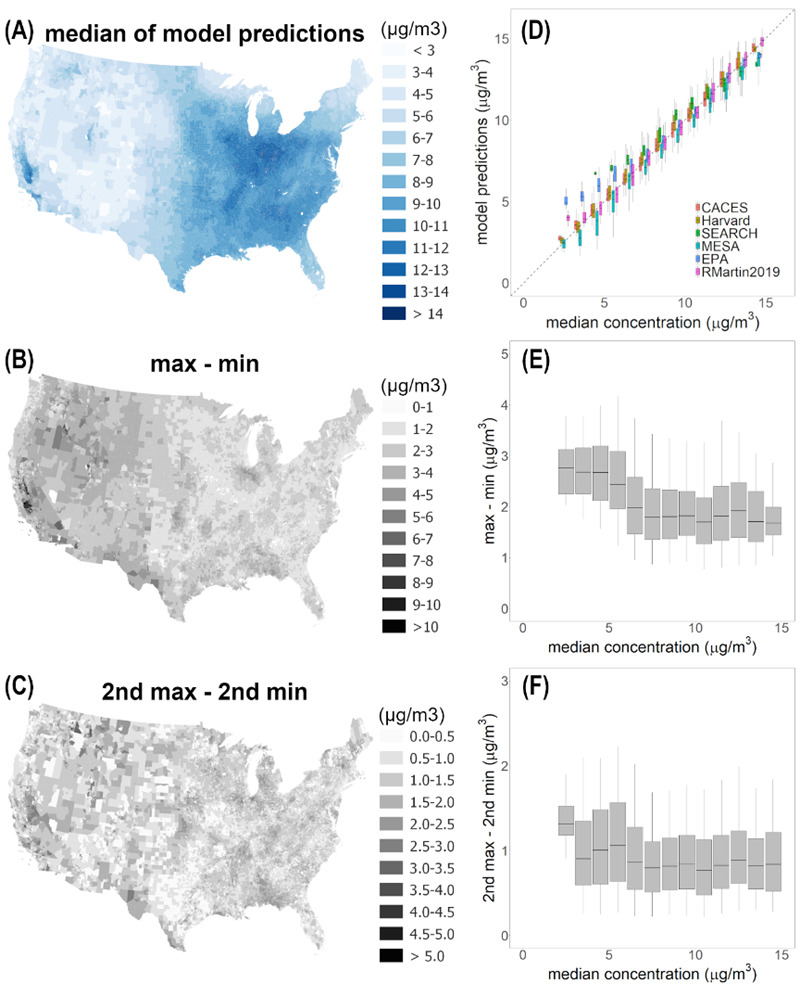
The amount of variability among predictions, when displayed separately by concentration and location (Figure 3) indicates relative agreement among the models, across the range of concentrations (Figure 3D). In locations for which the median predicted concentration is comparatively low (less than 6 μg/m3), EPA predictions tend to be slightly higher than the other models. For the very lowest-concentration locations (median predicted concentrations less than 3 μg/m3), the Martin2019 predictions too tend to be slightly larger than the other models. The SEARCH model is only available for the eastern half of the contiguous US and so therefore excludes lower-population-density, lower-concentration regions found in the western half of the contiguous US. The CACES and Harvard models tend to agree with each other and to be near the median prediction, for each concentration range (Figure 3D).

The range of model predictions (a measure of between-model disagreement) is approximately constant (in units of concentration rather than in, e.g., percent-difference; see Figure 3E, 3F) across levels of pollution, suggests additive rather than multiplicative errors. To the extent that there is a pattern (more so for Figure 3E than Figure 3F), the range of predictions is greater in lower- than in higher-concentration locations. The finding reflects the patterns mentioned in the previous paragraph: below 5 or 6 μg/m3, the EPA predictions (and, below 3 μg/m3, the Martin2019 predictions too) are larger than the other models’ predictions; it suggests that predicting concentrations in low-concentration locations might be more challenging (greater model-model difference) than in medium- or high-concentration locations.

Overall, our findings are generally consistent with hypothesis #1, not #2. Model-model comparisons can identify the level of model agreement/disagreement, but not of accuracy or error. In cases where the models agree (or disagree), it’s possible all of the models are incorrect. A useful step for future research would be to compare against held-out measurements — either via a coordinated effort by the researchers to hold out a consistent set of measurements, or via an independent dataset of concentrations that none of the researchers employed in model-building.

Text in the Supplemental Information (SI) provides background on this research, describes strengths and weaknesses, and documents that results here are relatively robust to several sensitivity analyses.

Figure 3
Figure 3.Variability by concentration and location.

Maps show median concentration among model predictions within each tract (A) and within-tract variability of model predictions calculated as the max minus min (B) and 2nd max minus 2nd min (C). Boxplots show (y-axis) range of tract-level model predictions (D) and within-tract variation calculated as either max minus the min (E) or 2nd max minus 2nd min (E) of model predictions within each tract as a function of the median concentration among model predictions within each tract, binned to 1 µg/m3 bins (x-axis). In the boxplots, horizontal bar shows the median, box shows the interquartile range, and vertical lines show the 5th and 95th percentiles of the variability for tracts within each bin.


Acknowledgements

We gratefully acknowledge the funders. This publication was developed as part of the Center for Air, Climate, and Energy Solutions (CACES), which was supported under Assistance Agreement No. R835873 awarded by the U.S. Environmental Protection Agency (EPA) for an Air, Climate, and Energy (ACE) center. Additional funding was from the EPA for the SEARCH ACE Center (RD83587101) and the Harvard-MIT ACE center (RD83479801). This manuscript has not been formally reviewed by EPA. The views expressed here are solely those of authors and do not necessarily reflect those of the Agency. EPA does not endorse any products or commercial services mentioned in this publication.

Submitted: October 19, 2023 AEST

Accepted: October 29, 2023 AEST

References

Di, Qian, Heresh Amini, Liuhua Shi, Itai Kloog, Rachel Silvern, James Kelly, M. Benjamin Sabath, et al. 2019a. “An Ensemble-Based Model of PM2.5 Concentration across the Contiguous United States with High Spatiotemporal Resolution.” Environment International 130 (September):104909. https:/​/​doi.org/​10.1016/​j.envint.2019.104909.
Google ScholarPubMed CentralPubMed
———. 2019b. “Assessing NO2 Concentration and Model Uncertainty with High Spatiotemporal Resolution across the Contiguous United States Using Ensemble Model Averaging.” Environmental Science & Technology 54 (3): 1372–84. https:/​/​doi.org/​10.1021/​acs.est.9b03358.
Google ScholarPubMed CentralPubMed
Goldberg, Daniel L., Pawan Gupta, Kai Wang, Chinmay Jena, Yang Zhang, Zifeng Lu, and David G. Streets. 2019. “Using Gap-Filled MAIAC AOD and WRF-Chem to Estimate Daily PM2.5 Concentrations at 1 km Resolution in the Eastern United States.” Atmospheric Environment 199 (February):443–52. https:/​/​doi.org/​10.1016/​j.atmosenv.2018.11.049.
Google Scholar
Keller, Joshua P., Casey Olives, Sun-Young Kim, Lianne Sheppard, Paul D. Sampson, Adam A. Szpiro, Assaf P. Oron, Johan Lindström, Sverre Vedal, and Joel D. Kaufman. 2015. “A Unified Spatiotemporal Modeling Approach for Predicting Concentrations of Multiple Air Pollutants in the Multi-Ethnic Study of Atherosclerosis and Air Pollution.” Environmental Health Perspectives 123 (4): 301–9. https:/​/​doi.org/​10.1289/​ehp.1408145.
Google ScholarPubMed CentralPubMed
Kim, Sun-Young, Matthew Bechle, Steve Hankey, Lianne Sheppard, Adam A. Szpiro, and Julian D. Marshall. 2020. “Concentrations of Criteria Pollutants in the Contiguous U.S., 1979 – 2015: Role of Prediction Model Parsimony in Integrated Empirical Geographic Regression.” PLoS ONE 15 (2): e0228535. https:/​/​doi.org/​10.1371/​journal.pone.0228535.
Google ScholarPubMed CentralPubMed
Requia, Weeberb J., Qian Di, Rachel Silvern, James T. Kelly, Petros Koutrakis, Loretta J. Mickley, Melissa P. Sulprizio, Heresh Amini, Liuhua Shi, and Joel Schwartz. 2020. “An Ensemble Learning Approach for Estimating High Spatiotemporal Resolution of Ground-Level Ozone in the Contiguous United States.” Environmental Science & Technology 54 (18): 11037–47. https:/​/​doi.org/​10.1021/​acs.est.0c01791.
Google ScholarPubMed CentralPubMed
Sampson, Paul D., Mark Richards, Adam A. Szpiro, Silas Bergen, Lianne Sheppard, Timothy V. Larson, and Joel D. Kaufman. 2013. “A Regionalized National Universal Kriging Model Using Partial Least Squares Regression for Estimating Annual PM2.5 Concentrations in Epidemiology.” Atmospheric Environment 75 (August):383–92. https:/​/​doi.org/​10.1016/​j.atmosenv.2013.04.015.
Google ScholarPubMed CentralPubMed
US EPA. 2017. “Downscaler Model for Predicting Daily Air Pollution.” https:/​/​19january2017snapshot.epa.gov/​air-research/​downscaler-model-predicting-daily-air-pollution_.html.
———. 2022. “Fused Air Quality Surface Using Downscaling (FAQSD).” https:/​/​www.epa.gov/​hesc/​rsig-related-downloadable-data-files.
van Donkelaar, Aaron, Randall V. Martin, Chi Li, and Richard T. Burnett. 2019. “Regional Estimates of Chemical Composition of Fine Particulate Matter Using a Combined Geoscience-Statistical Method with Information from Satellites, Models, and Monitors.” Environmental Science & Technology 53 (5): 2595–2611. https:/​/​doi.org/​10.1021/​acs.est.8b06392.
Google Scholar
Young, Michael T., Matthew J. Bechle, Paul D. Sampson, Adam A. Szpiro, Julian D. Marshall, Lianne Sheppard, and Joel D. Kaufman. 2016. “Satellite-Based NO2 and Model Validation in a National Prediction Model Based on Universal Kriging and Land-Use Regression.” Environmental Science & Technology 50 (7): 3686–94. https:/​/​doi.org/​10.1021/​acs.est.5b05099.
Google ScholarPubMed CentralPubMed

This website uses cookies

We use cookies to enhance your experience and support COUNTER Metrics for transparent reporting of readership statistics. Cookie data is not sold to third parties or used for marketing purposes.

Powered by Scholastica, the modern academic journal management system