Loading [Contrib]/a11y/accessibility-menu.js

This website uses cookies

We use cookies to enhance your experience and support COUNTER Metrics for transparent reporting of readership statistics. Cookie data is not sold to third parties or used for marketing purposes.

Skip to main content
null
Findings
  • Menu
  • Articles
    • Energy Findings
    • Resilience Findings
    • Safety Findings
    • Transport Findings
    • Urban Findings
    • All
  • For Authors
  • Editorial Board
  • About
  • Blog
  • search
  • X (formerly Twitter) (opens in a new tab)
  • LinkedIn (opens in a new tab)
  • RSS feed (opens a modal with a link to feed)

RSS Feed

Enter the URL below into your favorite RSS reader.

https://findingspress.org/feed
ISSN 2652-8800
Transport Findings
January 16, 2026 AEST

How does Regional Air Pollution affect Pedestrian, Car, and Transit Use?

Prachanda Tiwari, Patrick A Singleton, Ph.D., Keunhyun Park, Ph.D.,
Air qualityTravel behaviorMultilevel modelingPedestrian volumesTraffic countsTransit ridership
Copyright Logoccby-sa-4.0 • https://doi.org/10.32866/001c.155021
Findings
Tiwari, Prachanda, Patrick A Singleton, and Keunhyun Park. 2026. “How Does Regional Air Pollution Affect Pedestrian, Car, and Transit Use?” Findings, January. https:/​/​doi.org/​10.32866/​001c.155021.
Download all (3)
  • Figure 1. Map of data collection locations in Cache County, Utah, United States
    Download
  • Figure 2. Maps showing posterior slopes for pedestrian volumes for (left) yellow (AQI = 51–100) and (right) orange (AQI = 101–150) days
    Download
  • Supplemental Information
    Download

Sorry, something went wrong. Please try again.

If this problem reoccurs, please contact Scholastica Support

Error message:

undefined

View more stats

Abstract

To examine how regional air pollution affects multimodal traffic volumes, we analyzed two years (2018–2019) of daily automobile traffic counts, estimated pedestrian volumes, and transit ridership in Cache County, Utah, United States. Multilevel models accounted for locational differences while controlling for weather and other temporal variables. When the air quality was poor, pedestrian volumes decreased, automobile traffic increased, and system-wide bus ridership showed no significant change. Walking declines were larger in neighborhoods with higher car ownership and smaller in areas with greater street connectivity and more commercial land use.

1. Questions

During episodes of regional air pollution—such as from smog or wildfire smoke—public health and transportation stakeholders try to induce travel behavior changes through air quality alerts (Teague, Zick, and Smith 2015; Cummings and Walker 2000). In response, do people (1) drive less to reduce emissions, (2) avoid exposure by walking less, or (3) carry on as usual?

Population-level analysis of multimodal traffic over time can provide an answer to these questions. Yet, most prior studies examine only one mode at a time (Acharya and Singleton 2022; Doubleday et al. 2021; Saberian, Heyes, and Rivers 2017; Tribby et al. 2013; Welch, Gu, and Kramer 2005), making it difficult to know whether mode use shifts and/or volumes fall across all modes. Similarly, although locational contexts likely shape responses, few studies have modeled spatial variations in air quality–traffic relationships.

To address these gaps, we ask two questions:

  1. What are the aggregate effects of regional air pollution levels on pedestrian volumes, automobile traffic volumes, and transit ridership?

  2. How do the air quality–traffic relationships vary across locations (spatial heterogeneity)?

2. Methods

The study area is Cache County, Utah, United States, with a 2020 population of 133,154. The high mountain valley’s bowl-shaped terrain contributes to episodes of regional air pollution, specifically high particulate matter concentrations caused by wintertime temperature inversions and summertime wildfire smoke. Prior to and during such events, Utah government agencies issue air quality alerts (Utah DEQ, 2022) and encourage people to carpool, trip-shift, ride public transit, and telework (UDOT, 2022). These messages are often shared in local media.

We assembled daily time series data, from January 2018 through December 2019, for the following key variables:

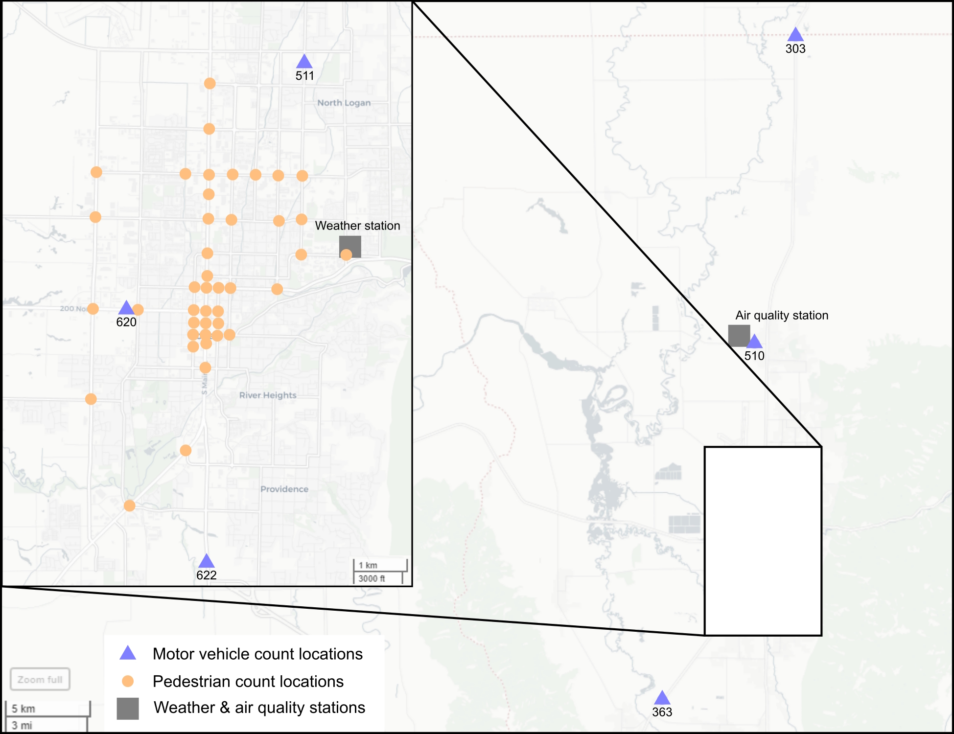
  • Daily pedestrian crossing volumes at 39 signalized intersections, estimated (Runa and Singleton 2021) from traffic signal push-button data.

  • Daily automobile traffic volumes at six continuous count stations operated by the Utah Department of Transportation.

  • System-wide daily bus boardings (no rail service) for the entire Cache Valley Transit District public transit system (no service on Sundays).

  • Daily air quality index (AQI) at one station, based on concentrations of fine particulate matter (PM2.5), from the U.S. Environmental Protection Agency. AQI was categorized by color: green = 0–50, yellow = 51–100, orange = 101–150, etc.

To address question 1, we estimated separate, mode-specific log-linear regression models of daily traffic, predicted by AQI category. We accounted for weather and other temporal effects by including control variables for precipitation, temperature, season, day-of-week, and holidays. To address question 2, we estimated these as multilevel (mixed effects) models, with daily observations nested within locations. For pedestrian volumes, we used random intercepts, predicted by built and social environment variables, and random AQI slopes; we also tested cross-level interactions to link slope variation to location characteristics. For automobile traffic volumes, we used fixed intercepts and fixed AQI slopes, due to the small number of locations (six). For transit ridership, we could not estimate multilevel models due to only having system-wide data.

Study locations are shown in Figure 1. Further details about the data and analyses, including descriptive statistics, are included in Supplemental Information.

Figure 1
Figure 1.Map of data collection locations in Cache County, Utah, United States

3. Findings

Table 1 presents results for question 1, about the aggregate effects of regional air pollution on multimodal traffic volumes.

Table 1.Aggregate effects of regional air pollution levels on multimodal traffic
Pedestrian volumesa Automobile traffic volumesb Transit ridershipc
Coefficients Estimate t-⁠statistic Estimate t-⁠statistic Estimate t-⁠statistic
Intercept 5.092a 32.356 9.060b 1207.460 8.686 332.388
Day of week (ref. = Weekday)
Saturday -0.366 -38.513 -0.122 -19.753 -1.245 -49.883
Sunday -1.020 -107.919 -0.614 -98.842 N/A N/A
Holiday (ref. = No holiday) -0.914 -49.317 -0.320 -27.073 -1.238 -18.829
Season (ref. = Winter)
Spring 0.266 24.874 0.097 14.267 -0.078 -2.512
Summer 0.373 36.192 0.135 19.693 -0.394 -13.292
Fall 0.361 34.074 0.109 16.172 0.057 1.839
Precipitation (ref. = No rain / no snow)
Light rain -0.060 -6.293 -0.021 -3.367 -0.032 -1.185
Heavy rain -0.157 -2.521 -0.024 -0.620 0.144 0.626
Light snow -0.259 -19.657 -0.062 -7.399 -0.069 -1.843
Heavy snow -0.341 -16.968 -0.123 -9.742 -0.041 -0.697
Max temperature (°C) difference from average 0.007 9.411 0.000 0.348 0.000 0.065
Air quality index (ref. = Green)
Yellow (AQI = 51–100) -0.053 -4.916 -0.003 -0.474 -0.017 -0.556
Orange (AQI = 101–150) -0.136 -5.929 0.049 3.333 -0.075 -1.186

a Random-intercept multilevel log-linear regression model. Overall N = 27,157 location–days, with 39 pedestrian volume intersections. Estimate shown is the mean intercept; the standard deviation of the intercept was 0.981.
b Fixed-intercept multilevel log-linear regression model. Overall N = 3,987 location–days, with six automobile traffic volume stations. Estimate shown is the intercept for one station; the estimated difference in intercept for other stations ranged from −0.663 (t = -91.996) to +1.084 (t = 147.750).
c Log-linear regression model. N = 608 days.
Notes: N/A = not applicable. Full model results are in Supplemental Information.

Overall, on days with worse air quality, pedestrian volumes decreased, automobile volumes increased, and bus ridership showed no significant change. Relative to green days, on average, pedestrian volumes were 5.2% lower on yellow days and 12.7% lower on orange days. This pattern is potentially explained by exposure-avoidance behavior: people walk less as AQI worsens. Compared to green days, on average, automobile traffic volumes were 5.1% higher on orange days, but not significantly different on yellow days. This increase with higher air pollution contradicts stakeholders’ hopes that air quality alerts reduce driving, but it is consistent with exposure-driven mode substitution behavior away from outdoor/active modes. System-wide bus boardings appeared to decrease slightly (by 7.2% on average) on orange days compared to green days, but this change was not statistically significant. Aggregate transit ridership responses may be limited by service design, trip purposes, or transit dependence.

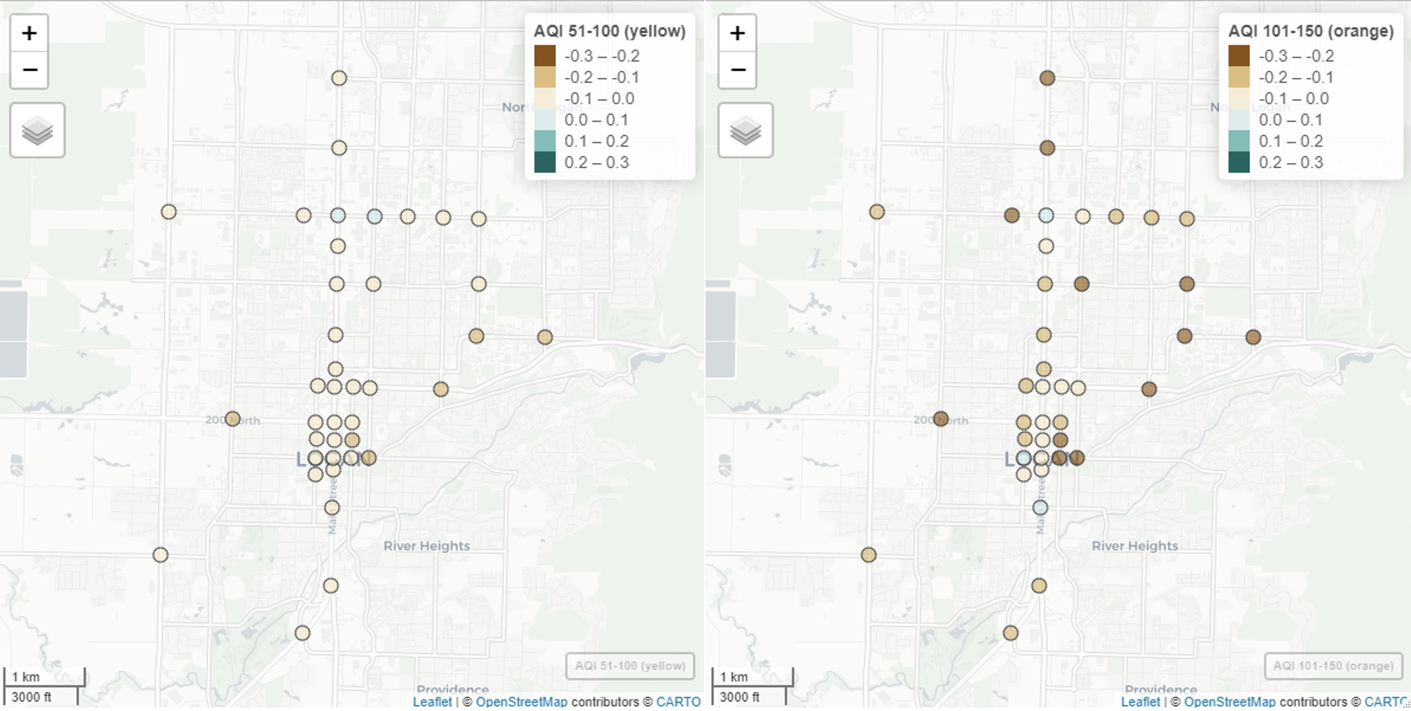
Figure 2 shows spatial variations in relationships between AQI and pedestrian volumes (specifically, posterior slopes (Snijders and Bosker 2012)), thus helping to address question 2. Locations with more negative coefficients—indicating a larger deterring effect of air pollution—seem to be located in more peripheral or suburban areas, including to the east near a university campus.

Figure 2
Figure 2.Maps showing posterior slopes for pedestrian volumes for (left) yellow (AQI = 51–100) and (right) orange (AQI = 101–150) days

Considering cross-level interactions with AQI, several built and social environment variables were significant in the pedestrian model. Higher car ownership led to larger pedestrian declines on higher pollution days (especially yellow), which is consistent with substitutions away from walking where cars are more available. Also, higher car ownership could signify higher income groups, who may tend to use cars on polluted days (Kim, Ko, and Jang 2023). Conversely, more commercial land led to smaller pedestrian declines on poor-air days (yellow), consistent with walkable destinations being closer and trip necessity higher in mixed-use areas. Similarly, in areas with greater street connectivity (share of 4-way intersections), we found smaller pedestrian declines on orange days, consistent with resilient pedestrian networks supporting shorter, more direct trips even when air quality is worse (Tal and Handy 2012).

For automobile traffic volumes, we did not find significant spatial variations in the AQI slope, potentially because there were only six stations. We could not evaluate spatial heterogeneity in transit ridership because only system-wide data were available.

In summary, observed patterns in this study region suggest that current strategies like air quality alerts are not reducing driving; instead, people are driving more and walking less. To encourage more healthy travel behavior change during episodes of regional air pollution, stronger policies may be required, such as mandatory employer-based programs like carpooling or telework.


Acknowledgements

This work was conducted with support from Utah State University and the Mountain-Plains Consortium, a University Transportation Center funded by the U.S. Department of Transportation. The contents of this paper reflect the views of the authors, who are responsible for the facts and accuracy of the information presented.

Submitted: December 04, 2025 AEST

Accepted: January 07, 2026 AEST

References

Acharya, S., and P. A. Singleton. 2022. “Associations of Inclement Weather and Poor Air Quality with Non-Motorized Trail Volumes.” Transportation Research Part D: Transport and Environment 109:103337. https:/​/​doi.org/​10.1016/​j.trd.2022.103337.
Google Scholar
Cummings, R. G., and M. B. Walker. 2000. “Measuring the Effectiveness of Voluntary Emission Reduction Programmes.” Applied Economics 32 (13): 1719–26. https:/​/​doi.org/​10.1080/​000368400421066.
Google Scholar
Doubleday, A., Y. Choe, T. M. Busch Isaksen, and N. A. Errett. 2021. “Urban Bike and Pedestrian Activity Impacts from Wildfire Smoke Events in Seattle, WA.” Journal of Transport & Health 21:101033. https:/​/​doi.org/​10.1016/​j.jth.2021.
Google Scholar
Kim, S., Y. Ko, and K. Jang. 2023. “Role of Income on Travel Behavior in Polluted Air.” Journal of Transport & Health 33:101705. https:/​/​doi.org/​10.1016/​j.jth.2023.101705.
Google Scholar
Runa, F., and P. A. Singleton. 2021. “Assessing the Impacts of Weather on Pedestrian Signal Activity at 49 Signalized Intersections in Northern Utah.” Transportation Research Record: Journal of the Transportation Research Board 2675 (6): 0361198121994111. https:/​/​doi.org/​10.1177/​0361198121994111.
Google Scholar
Saberian, S., A. Heyes, and N. Rivers. 2017. “Alerts Work! Air Quality Warnings and Cycling.” Resource and Energy Economics 49:165–85. https:/​/​doi.org/​10.1016/​j.reseneeco.2017.05.004.
Google Scholar
Snijders, T. A. B., and R. J. Bosker. 2012. Multilevel Analysis: An Introduction to Basic and Advanced Multilevel Modeling. Sage.
Google Scholar
Tal, G., and S. Handy. 2012. “Measuring Nonmotorized Accessibility and Connectivity in a Robust Pedestrian Network.” Transportation Research Record: Journal of the Transportation Research Board 2299 (1): 48–56. https:/​/​doi.org/​10.3141/​2299-06.
Google Scholar
Teague, W. S., C. D. Zick, and K. R. Smith. 2015. “Soft Transport Policies and Ground-Level Ozone: An Evaluation of the ‘Clear the Air Challenge’ in Salt Lake City.” Policy Studies Journal 43 (3): 399–415. https:/​/​doi.org/​10.1111/​psj.12105.
Google Scholar
Tribby, C. P., H. J. Miller, Y. Song, and K. R. Smith. 2013. “Do Air Quality Alerts Reduce Traffic? An Analysis of Traffic Data from the Salt Lake City Metropolitan Area, Utah, USA.” Transport Policy 30:173–85. https:/​/​doi.org/​10.1016/​j.tranpol.2013.09.012.
Google Scholar
Utah Department of Environmental Quality (Utah DEQ). 2022. “Air Quality Forecast: Forecast Legend.” https:/​/​air.utah.gov/​forecastLegendAQI.html.
Utah Department of Transportation (UDOT). 2022. “TravelWise: Rethink Your Trip.” https:/​/​travelwise.utah.gov/​.
Welch, E., X. Gu, and L. Kramer. 2005. “The Effects of Ozone Action Day Public Advisories on Train Ridership in Chicago.” Transportation Research Part D: Transport and Environment 10 (6): 445–58. https:/​/​doi.org/​10.1016/​j.trd.2005.06.002.
Google Scholar

Powered by Scholastica, the modern academic journal management system