1. Questions
Hansen (1959) established the weighted-sum structure of generalized cost components (e.g., time, money, operating costs) that underlies many access indices. In practice, analysts must pick an impedance (e.g., a cumulative threshold (all opportunities within equally counted), an exponential decay or an inverse power
We ask:
-
When do different impedances yield the same percentage changes in access under uniform changes in land use, speed, or time budget?
-
When are cross-place rankings independent of the impedance?
-
How do these conditions relate to the frequent empirical finding that cumulative and gravity-type metrics are highly correlated?
Empirically, many studies report that common access measures often yield similar rankings or conclusions under typical parameter choices (Santana Palacios and El-Geneidy 2022; Kapatsila et al. 2023; Vale and Pereira 2017). This motivates the hypothesis that, under mild conditions, impedance choice may be irrelevant in specific senses. However, the precise reasons for this robustness have not been formally established. This paper sharpens and extends earlier insights by deriving general analytic results. We provide explicit elasticity formulas for accessibility with respect to uniform changes in land-use density, travel speed, and time budget, showing how these sensitivities compare across impedance functions (building on the qualitative trade-offs noted by Levine et al. (2012)). We also introduce a new decomposition of Hansen’s index into discrete distance-band contributions, which offers a clearer interpretation of how different decay functions weight near vs. far opportunities. Finally, we identify a simple dominance condition – proportional cumulative opportunity curves across locations – under which any impedance choice will yield identical cross-place accessibility rankings. This theoretical condition helps explain the empirical findings of prior work that different accessibility metrics often lead to the same conclusions. In these ways, our paper formalises and generalises scattered observations from the literature, providing a stronger foundation for when impedance choices are truly irrelevant and when they might matter.
2. Methods
Note: A complete nomenclature table is provided in Table 1.
We work with travel cost or time, denoted or for arguments and budgets, respectively. Here, ‘budget’ means a time or generalised cost limit or threshold, not monetary expenditure. Let be generalised cost from origin to opportunity and the size of opportunity
Hansen’s primal accessibility with budget is given by
\[A_i(T; f) = \sum_{j: c_{ij}\le T} O_j f(c_{ij}). \tag{1}\]
We use this budgeted form for all impedances. While an unbudgeted sum exists when in the uniform–plane benchmark, which assumes constant speed across space (no congestion or signals), discrete sums are typically budgeted in practice, using the cumulative curve defined as the sum of opportunities that can be reached from within travel cost :
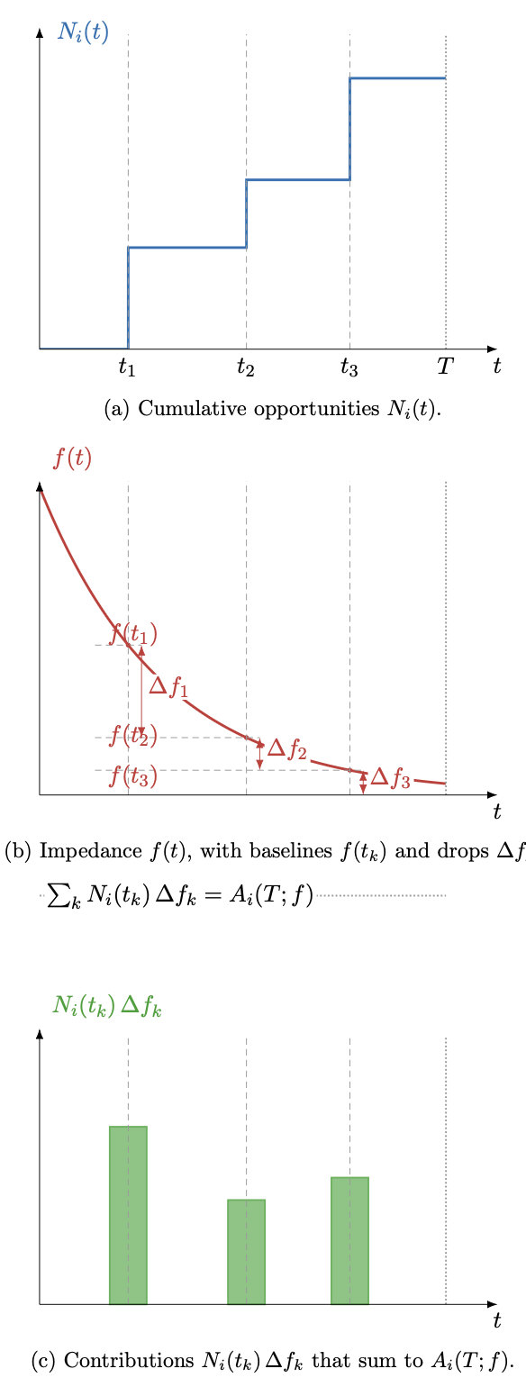
\[N_i(t) = \sum_{j: c_{ij}\le t} O_j. \tag{2}\]
Discrete jump-sum identity. The jump–sum identity says that accessibility can be computed as the sum, over each travel-time threshold, of the cumulative number of reachable opportunities at that threshold multiplied by the drop in the impedance weight at that point. Formally: Assume is non–increasing, bounded, and right–continuous with so is well defined. Let be the strictly increasing ordering of the distinct costs where jumps, with jumps and set Define with Then
\[A_i(T; f) = \sum_{k: t_k\le T} N_i(t_k) \,\Delta f_k. \tag{3}\]
Note: Any tie–breaking that preserves the cumulative steps yields the same since only and enter Equation (3). The jump-sum identity is shown in Appendix A.
Because is non-increasing, the framework excludes cases where being closer is undesirable (e.g., noise/safety next to certain stops).
Uniform-plane benchmark. The uniform-plane benchmark assumes opportunities are spread evenly across space and travel occurs at constant speed, so accessibility reduces to integrating opportunity density over concentric circles around an origin. Formally: for a uniform planar density and speed the marginal annulus area at time is proportional to so
\[A_i(T; f) = 2\pi\rho v^2 \int_{0}^{T} t\,f(t)\,\mathrm{d}t. \tag{4}\]
This gives the elasticities
\[E_\rho = 1,\qquad E_v = 2,\qquad E_T(T; f) = \frac{T^2 f(T)}{\displaystyle\int_{0}^{T} t\,f(t)\,\mathrm{d}t}. \tag{5}\]
Ranking invariance across impedances. If the cumulative opportunity curves for two places are proportional at all travel times, then their accessibility rankings will be the same no matter which impedance function is used. More precisely: if cumulative curves are proportional across places, for all then for any non-increasing with
\[A_i(T; f) = \alpha_i \sum_{k: t_k\le T} N^\star(t_k) \,\Delta f_k, \tag{6}\]
so if and only if independent of
3. Findings
We next discuss the Findings in order.
Three results explain when impedance choice matters:
-
First, in a uniform planar benchmark, density and speed elasticities are invariant across impedances.
-
Second, cumulative opportunities is the only such impedance function with a constant time elasticity. See Eq. (7).
-
Third, if cumulative curves are proportional across places, cross–place rankings do not depend on the impedance.
F1. Elasticity equivalence for land use and speed. On the uniform plane (see Methods, Section 2), the marginal annulus area at time is proportional to implying E E (see Eq. (5)).
These invariances rely on the uniform-plane benchmark; strong spatial non-uniformity or network effects can break them.
F2. Constant time elasticity. Among the canonical impedances shown here, only the cumulative opportunities has constant. For cumulative opportunities
\[A=\pi\rho v^2 T^2,\qquad E_T={2} \,\, \forall \,\,T. \tag{7}\]
Other impedances have that varies with determined by the tail of
F3. Ranking invariance across impedances. If cumulative curves are proportional across places, for all then for any non-increasing with
\[A_i(T; f) = \alpha_i \sum_{k: t_k\le T} N^\star(t_k)\,\Delta f_k, \tag{8}\]
so if and only if independent of
To diagnose whether this holds: plot for competing places over nearly parallel curves indicate ranking stability across impedances, while crossings signal possible ranking flips as or varies.
F4. Practical indifference in narrow bands. When relevant travel times concentrate near a typical many impedances are nearly flat on that band, so percentage responses and rankings are often locally similar.
Illustration on the uniform plane. Three canonical impedances give closed forms with compact displays. Cumulative :
\[A=\pi\rho v^2 T^2,\qquad E_T=2. \tag{9}\]
Exponential where denotes the exponential decay parameter:
\[\begin{aligned} A &= \frac{2\pi\rho v^2}{\theta^2}\Bigl[1-(1+\theta T)e^{-\theta T}\Bigr],\\ E_T(T; e^{-\theta\cdot}) &= \frac{\theta^{2}T^{2}e^{-\theta T}}{1-(1+\theta T)e^{-\theta T}}. \end{aligned}\tag{10}\]
The micro-cutoff is the smallest practical time considered, used to avoid singularities at Inverse–square with micro–cutoff :
\[A=2\pi\rho v^2\,t_0^2 \ln\!\frac{T}{t_0},\qquad E_T(T;f)=\frac{1}{\ln(T/t_0)}. \tag{11}\]
In all three cases and (see Eq. (5)).
When equivalence fails. See Supplemental Information for worked examples. Ranking invariance requires for all If curves cross, weights on near versus far thresholds matter and different can reverse rankings, and thus interpretations. Time–elasticity invariance relies on the planar annulus area being proportional to so non-uniform density or network effects can break it.
)_with_three_cost_thresholds__.jpg)
A. Supplemental Information: Examples
A.1. Ranking flip threshold (what makes rankings change?)
Motivation. The main text shows when rankings are invariant. This example isolates the opposite case, when two places can swap order as the impedance shifts attention from near to far opportunities.
Place A has opportunities at cost and at cost Place B has at and at With the exponential impedance
\[A_A(\theta) - A_B(\theta) = (N_{A,\text{near}} - N_{B,\text{near}}) e^{-\theta a} + (N_{A,\text{far}} - N_{B,\text{far}}) e^{-\theta b}. \tag{12}\]
If the near advantage favors A and the far advantage favors B,
\[N_{A,\text{near}} > N_{B,\text{near}},\qquad N_{A,\text{far}} < N_{B,\text{far}}, \tag{13}\]
to ensure require then there is a unique threshold where the ranking flips,
\[\theta^\ast = \frac{1}{b - a}\ln\!\left(\frac{N_{B,\text{far}} - N_{A,\text{far}}}{N_{A,\text{near}} - N_{B,\text{near}}}\right). \tag{14}\]
For the near opportunities dominate and for the far opportunities dominate and
For the cumulative impedance with budget the ranking is piecewise by threshold: if both are zero, if the near counts decide, if the near plus far counts decide.
A.2. When different impedances give almost the same answer
Motivation. Practitioners often care about a specific time range, for example typical peak travel times. Many common impedances place most of their weight on that range. If two places look similar within that range, their access scores will be nearly proportional, no matter which such impedance is used.
Let the times where another opportunity becomes reachable be up to budget and write the discrete representation
\[\begin{aligned} A_i(T; f) &= \sum_{k: t_k\le T} N_i(t_k) \,\Delta f_k,\\ \Delta f_k &= f(t_k) - f(t_{k+1}),\\ f(\infty) &= 0. \end{aligned}\tag{15}\]
Fix a time range of interest and split the sum into inside and outside that range,
\[A_i(T; f) = \underbrace{\sum_{t_k\in[a,b]} N_i(t_k) \,\Delta f_k}_{\text{in range}}+\underbrace{\sum_{t_k\in/[a,b]} N_i(t_k) \,\Delta f_k}_{\text{outside range}}. \tag{16}\]
When an impedance concentrates on a time range where the places look alike, different impedances make little difference to the comparison. More formally:
If most of the impedance weight lies in
\[\sum_{t_k\in/[a,b]} \Delta f_k \le \varepsilon \quad \text{with small }\varepsilon, \tag{17}\]
and the two places have approximately proportional cumulative curves on that same range,
\[N_A(t) \approx \alpha N_B(t)\quad \forall t \in [a,b], \tag{18}\]
then their scores are nearly proportional,
\[A_A(T; f) \approx \alpha\, A_B(T; f). \tag{19}\]
This leaves a discrepancy no larger than times a bound on the cumulative counts.