RESEARCH QUESTIONS & HYPOTHESES

Transit agencies and transport planners are increasingly considering social equity as an important planning objective. However, there is little existing work on creating clearly defined benchmarks which can be used to evaluate the current state of transport equity in cities, assess the effectiveness of new transport plans, or in retrospect, analyze whether there have been improvements or declines in equity over time (Manaugh, Badami, and El-Geneidy 2015; Karner and Niemeier 2013).

Theoretically, measures of social equity in transport can be classified into measures of horizontal equity, how evenly transport costs and benefits are meted out across the overall population, and measures of vertical equity, how costs and benefits are distributed according to socio-economic status (e.g. by income group). Social equity in transport can also pertain to differences in opportunity (e.g. transit availability, auto-ownership) or differences in outcomes (e.g. travel distances, activity participation rates) (Bannister 2018).

Our primary objective is to find what the existing state of transit equity is in the GTHA across these dimensions (horizontal and vertical, opportunity and outcome). We use a regional travel survey to derive a series of simple and intuitive equity measures designed to be easily repeatable for future waves of the travel survey, or for other urban areas with similar available data.

DATA & METHODS

Our primary data comes from the 2016 Transportation Tomorrow Survey (TTS) (Data Management Group 2016). This survey is a 5% sample and contains a one-day travel diary for everyone aged 11 years and older (n = 269,770). The data includes a vector of expansion weights that can be used to estimate population-level equity metrics (N = 5,933,924). We also use a measure of transit access to jobs as a proxy for the transit provision available to each survey respondent. This measure sums the number of jobs reachable from a neighbourhood by public transit, weighting nearby jobs more than those further away.

$$A_{i} = \sum_{j = 1}^{J}{O_{j}\ (180\left( 90 + t_{i,j} \right)^{- 1} - 1)}$$

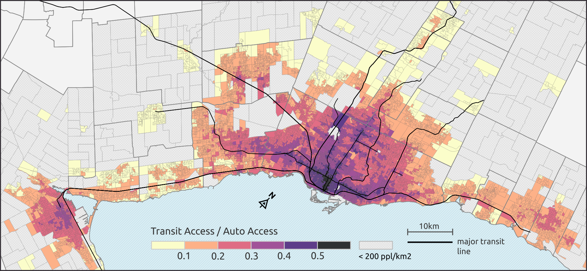
where $A_{i}$ is the accessibility score for a zone i, $O_{j}$ is the number of jobs in zone j, and $t_{i,j}$ is the transit travel time from i to j in minutes. In the equation, a job takes a weight of 1 if the travel time is 0, and a value of 0 if the travel time is 90 minutes or more. $A_{i}$ is computed as an overall score, as well as relative to the level of access to jobs by car for each neighbourhood. Specific details on how the accessibility measures were computed can be found in a technical report (Allen and Farber 2018). Figure 1 displays a map of relative transit accessibility in the region. The accessibility scores are computed at the Statistics Canada Dissemination Area unit of geography.

Figure 1 - Ratio of transit access to auto access to jobs in the GTHA

We use two measures of horizontal equity that can describe and keep track of the evenness of transport provision and outcomes. The first is the coefficient of variation (CV), which is a standardized measure of dispersion, computed as the standard deviation divided by the mean; the greater the CV, the more unevenness in the quantities being measured. Secondly, we compute Gini coefficients. The Gini coefficient ranges between 0 and 1, where 0 expresses perfect equality when all values are the same, and 1 expresses maximal unevenness when one individual (or zone) has all of the good being distributed. The Gini coefficient has been used previously in transport equity studies in other cities such as Melbourne, Australia (Delbosc and Currie 2011).

We measure vertical equity comparing between social groups with a ratio (Bannister 2018). For example, the ratio of mean activity participation rates of low-income households to high-income households is a telling measure of how inequitably participation is achieved by people with different income levels. For this paper, we provide ratios according to household income, car-ownership per household, and age. There are other socio-economic status (SES) groups like visible minorities, recent immigrants, or the disabled, which could be analyzed similarly. However, the TTS does not include variables for these groups, so they are not analyzed at this juncture.

Another important vertical equity benchmark to keep track of is the accounting of transport poverty, i.e. how many people are both transport disadvantaged and socially disadvantaged. We achieve this by estimating the number of low SES individuals that are also living in low-accessibility neighbourhoods in the region. Similar work was conducted in Canada using data from the Canadian census (Allen and Farber 2019), but was limited by a high level of aggregation, and not having data on car-ownership, a key indicator of transit dependence (car-ownership is not included in the Canadian census).

FINDINGS

Table 1 displays measures of horizontal equity. Overall, accessibility, trips, and activities display moderate levels of unevenness, while participation in discretionary activities is highly uneven. Achieving evenness through the removal of benefits at the high-end of accessibility makes little policy sense, but if evenness is attained by uplifting those on the lowest end of the spectrum, then achieving greater levels of horizontal equity can be interpreted positively.

Table 2 provides the vertical equity measures. We find that households with low-incomes and no cars tend to live in neighbourhoods with greater levels of transit accessibility, but take fewer trips per day, and participate in fewer daily activities. We also find that low-income and zero-car households travel shorter distances than their affluent counterparts, but travel times are much closer between groups. This is an indication that lower SES groups travel at slower speeds using non-auto modes. For age, youth live in areas with lower levels of transit accessibility than adults. As well, despite trips and overall activities nearly being equal between youth and adults, youth perform only half the number of discretionary activities. Middle-aged conduct more trips and more overall activities compared to the elderly, but only about ¾ the number of discretionary activities.

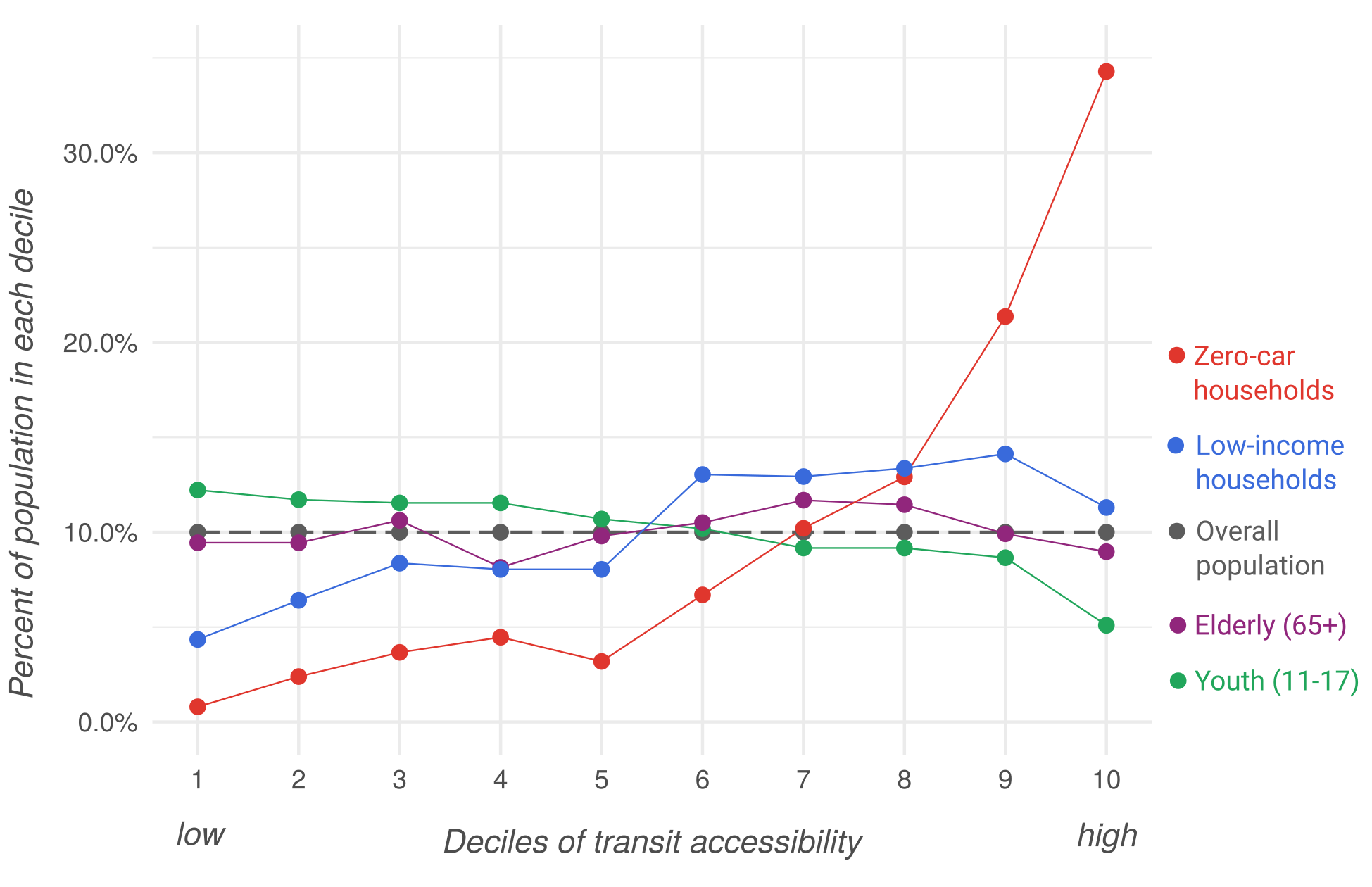
Table 3 presents counts of individuals living within each decile of transit accessibility, and each category of absolute accessibility by 100,000 job intervals. The percent of each population segment that falls within each decile or interval is displayed in Figures 2 and 3, respectively. In general, youth are more likely to live in low-access areas while car-free and low-income households are more likely to reside in areas of relatively higher access. Despite this trend, there are still 274k people in low-income households who live in areas of low transit accessibility (<100k jobs). This amounts to 30% of all individuals living in low-income households. The spatial locations of low-income households in relation to transit accessibility can be viewed on an interactive map at https://sausy-lab.github.io/canada-transit-access/map.html.

Figure 2 - Percent of population by decile of transit accessibility

Figure 3 - Percent of population by equal interval of transit accessibility

ACKNOWLEDGMENTS

We thank Metrolinx for providing financial support for this research.