RESEARCH QUESTION AND HYPOTHESIS
The value of travel time savings is defined as the marginal rate of substitution between travel cost and reductions in travel time (i.e., savings). The value of travel time reliability is the marginal rate of substitution between travel cost and increases in the predictability (i.e., reducing the variability) of travel time. It is typically quantified using one of two frameworks: centrality-dispersion (or mean-variance) (Jackson and Jucker 1982) and scheduling delays under uncertainty (Noland and Small 1995; Small 1982). Centrality-dispersion is based on the idea that the travel time unreliability (or variability) is concentrated in a statistical measure of the dispersion of the travel time distribution. The scheduling delay approach assumes that travelers have a specified time of arrival, and any expected late arrivals or expected early arrivals incur disutility. These disutilities are asymmetric, in contrast to the centrality-dispersion framework, which assumes all disutilities (due to unreliability) are weighted equally. It should be noted that expected refers to the first statistical moment of schedule delays due to late arrivals or early arrivals over the travel time distribution (Carrion and Levinson 2012b).
The ratio between these values is known as the reliability ratio. This study aims to systematically compare estimated reliability ratios using self-reported (perceived or subjective) travel times from surveys and measured (actual or objective) travel times by GPS devices. Extending the literature on measurement errors [@7959; @7963; @7968; @7969; @7970; (Parthasarathi, Levinson, and Hochmair 2013; Peer et al. 2014; Varela, Börjesson, and Daly 2018; Varotto et al. 2017; Vreeswijk et al. 2014) we posit that these values are different and that perceived times will produce a higher reliability ratio than measured times.
METHODS AND DATA
The data used were collected during previous research efforts (Carrion and Levinson 2012a; Zhu 2010). These studies aimed to understand the behavior of travelers due to the collapse of the I-35W bridge (August 1, 2007) and the opening of the bridge’s replacement to the public (September 18, 2008) in the Minneapolis–St. Paul region. The data consist of GPS observations and web-based surveys collected before and after the replacement bridge opened. A total of 97 subjects had usable, complete day-to-day GPS and survey data. For this study, only 39 subjects had sufficient observations on both interstate and noninterstate bridges.
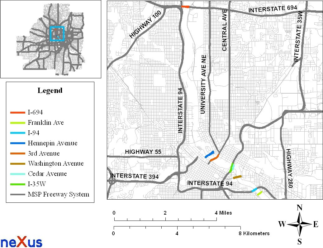
Table 1 summarizes the sociodemographic information of the subjects. The sample differs from the population of the Minneapolis–St. Paul region in several ways: Subjects are older, are more educated, and have a more uniform distribution of income.
In this study, the dataset was analyzed through random utility models (Ben-Akiva and Lerman 1985; Ortuzar and Willumsen 2011; Train 2009) The dataset is composed of two observations (home-to-work and work-to-home) for each of 39 subjects, yielding a total of 78 observations. Centrality and dispersion measures were calculated on the travel time distributions and were included as attributes in the systematic utilities of the random utility models.
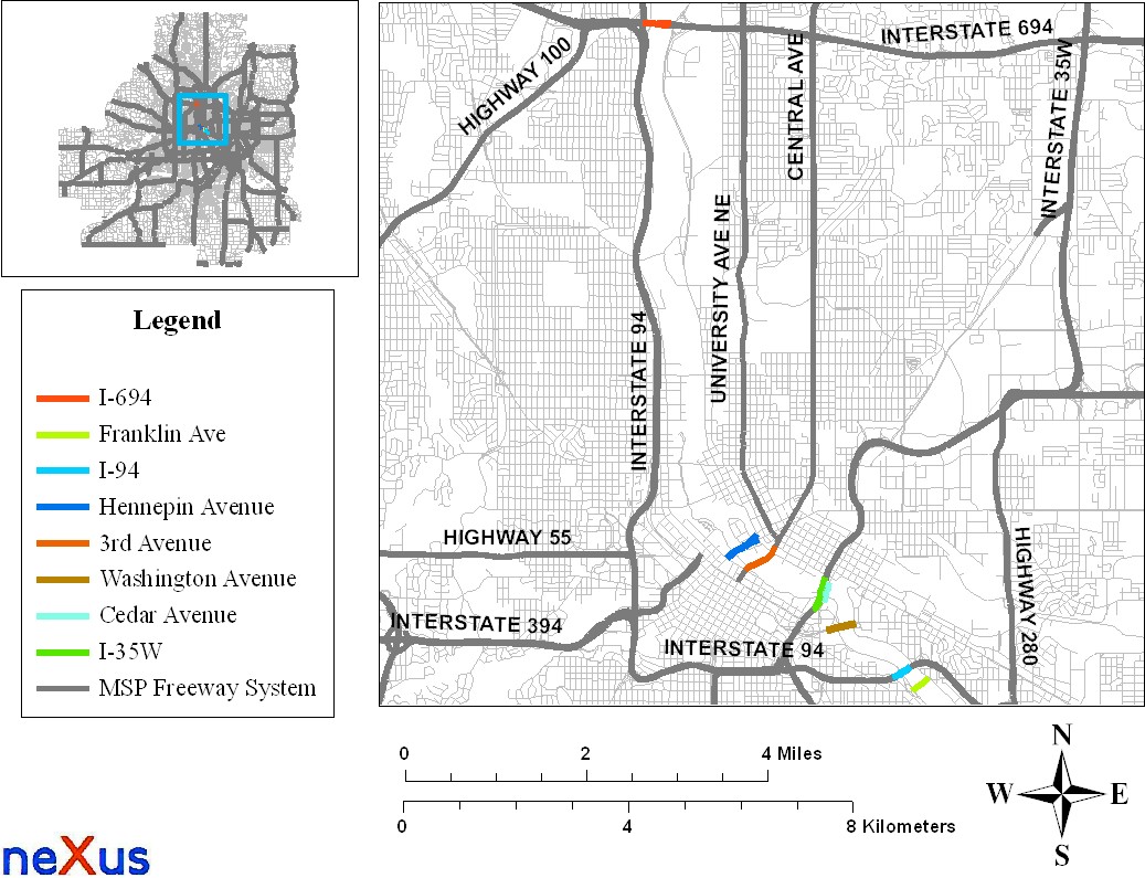
The choice dimension was based on the hierarchy of the bridges (interstate, noninterstate) across the Mississippi River (see Figure 1). Thus, the set of home-to-work trips and the set of work-to-home trips were further disaggregated to two alternatives (or choices). The first alternative represents the most used (i.e., highest number of commuter trips) bridge that belonged to the interstate category, and the second alternative represents the most used bridge that belonged to the noninterstate category. The bridge with the smallest travel time by centrality and dispersion measures was selected if two or more bridges had the same number of commute trips. Furthermore, a bridge was considered chosen by a subject if the number of trips on the bridge was strictly higher compared to the alternative. A binomial logit model was estimated following standard procedures (Train 2009). The confidence intervals for the reliability ratio of the models were calculated using the delta method (Cramer 1986; Greene 2012; Johnston and DiNardo 1997).
The additive linear-in-parameters systematic utility for the alternatives for all models was:
(1)
where:
-
Centrality measures of travel time (T ) (minutes) were calculated for the travel time distributions for the set of home-to-work and work-to-home trips for each alternative per subject (for this study, the mean and the median were considered centrality measures);
-
Dispersion measures of travel time (V) (minutes) were calculated for the travel time distributions for each trip for each alternative per subject (for this study, the standard deviation, a typical measure in the centrality-dispersion framework, and the difference between the 90th percentile and the median were considered dispersion measures);
-
Gender (G) was set to 1 = Male and 0 = Female based on participant responses from the web survey;
-
Income (I) was divided into four categories: ([$0, $49,999], [$50,000, $74,999], [$75,000, $99,999], and [$100,000, ∞+]), with the first category as the base case (in 2008 US dollars);
-
Type of work trip (D) was set to 1= trip originates from home and 0 = from work; and
-
Alternative specific constants (A) of the interstate alternative was set to 0.
FINDINGS
Table 2 presents the estimates of the random utility models (binomial logits), along with the reliability ratios and goodness-of-fit statistics. There were four types of models estimated according to distinct centrality and dispersion measures of travel time: mean/standard deviation (SD); mean/difference between 90th percentile and median (DMP90); median/SD; and median/DMP90. The four types of models were estimated with self-reported travel times from surveys and with measured travel times from GPS devices. The results indicate that the estimates of the centrality and dispersion measures of travel times are negative and highly statistically significant across all models. The goodness-of-fit statistics indicate that the models with self-reported travel times from surveys fit the data better than models with measured travel times from GPS devices. Both the Akaike information criterion and the Bayesian information criterion favor the models with self-reported travel times over the models with measured travel times. Thus, the models estimated with self-reported travel times are preferred on a statistical basis, and more specifically the mean/SD model.
The reliability ratios in the models with self-reported travel times were higher than one, except for the mean/DMP90 model. The 95% confidence intervals of these models indicate that values greater than one are more plausible. In contrast, the reliability ratios in the models with measured travel were less than one. The 95% confidence intervals of these models indicate that values less than one are more plausible. In addition, there were few overlaps of the 95% confidence intervals for the same models with self-reported travel times versus measured travel times. This is an important finding, as it gives different results with regard to the subjects’ valuing of travel time savings and travel time reliability.
The centrality-dispersion models with self-reported travel times indicate that the subjects generally value the travel time variability over the expected travel time. In contrast, the centrality-dispersion models with measured travel times indicate that the subjects value expected travel time over the travel time variability. Therefore, questions arise about which of the travel times (self-reported or measured) should be trusted.
It is known that perception error is a factor that distorts the traveler’s interpretation of actual travel times. It is likely that travelers execute their travel decisions based on their perceived travel times and not the actual travel times. This perception also is linked to the valuation of travel time, and thus the reliability ratios may be inflated or deflated depending on the level of distortion or magnitude of the perception error.
Lastly, the sociodemographic (e.g., income and gender) and type of work trip variables were not found statistically significant. Thus, the subjects were more influenced by the travel time measures in their choices. This result corroborates work by (U.S. Census Bureau 2008), which used the same data source, albeit not the exact same dataset.
ACKNOWLEDGMENTS
This study was supported by the Oregon Transportation Research and Education Consortium (2008-130 Value of Reliability and 2009-248 Value of Reliability Phase II) and the Minnesota DOT project “Traffic Flow and Road User Impacts of the Collapse of the I-35W Bridge over the Mississippi River.” We would also like to thank Kathleen Harder, John Bloomfield, and Shanjiang Zhu.