1. Questions

Climate-conscious consumers can reduce their carbon footprint by implementing load reduction and load shift measures to minimize the emissions caused by their energy consumption. Retail consumers are usually served by utilities who procure energy from various sources while minimizing cost. The emissions impact of reduced energy consumption is through the marginal resource, which is often the most expensive generation source (WattTime 2022).

The marginal emissions intensity of energy generation can be defined as the carbon emissions (lbs. CO\(_2\)) produced per unit of energy generated (measured in MWh). It varies significantly across time of day and year, which then affects the emissions impact of reduced energy consumption (Graff Zivin, Kotchen, and Mansur 2014). Researchers have studied the aggregate impact of repeated load shift measures using marginal emissions intensity data (Carmichael et al. 2021), and found that load flexibility can help reduce emissions significantly.

However, load shift/shed measures are expensive—they cause discomfort to building occupants, and require either manual intervention or investment in automated equipment. For loads which can not be shifted or shed repeatedly, we need to prioritize interventions which can achieve the highest emissions reduction by understanding the time-varying nature of marginal emissions intensity. Our research question is: do a few time periods in the year have an outsize potential to reduce emissions?

2. Methods

We use data on the emissions intensity of electricity consumption from WattTime (WattTime 2023), and data on electricity consumption of residential consumers using simulated end-use load profiles from a study by NREL (Frick et al. 2019). We validate the robustness of our findings with marginal emissions data from the PJM market operator region (PJM 2023).

Marginal Emissions Intensity

Marginal emissions intensity is characterized by the Marginal Operating Emissions Rate (MOER), and is measured in lbs. of CO\(_2\) emitted per MWh of energy generated. We use the WattTime API (WattTime 2023) to access historical MOER for the Northern Californian grid for 2018–2021, reported at 5-minute intervals and calculated using empirical modeling of the power system. WattTime uses a combination of models including heat rate models and grid operator dispatch models which aim to identify the marginal resource and then use its emissions intensity (WattTime 2022). MOER values typically range between 800–1200 lbs. CO\(_2\) per MWh.

The MOER exhibits spikes, and shifting and shedding load around these times can be particularly effective for reducing emissions. A quantity of interest for us is the MOER differential, i.e., the maximum MOER decrease possible within \(\pm 1\) hour of the time period under consideration, which can be interpreted as the emissions reduction possible if one unit of energy consumption can be shifted to any time up to one hour before or after the time period under consideration.

We analyze time periods when either the MOER or MOER differential is particularly high, in order to increase the effectiveness of load shed or shift actions. We rank time periods based on these parameters, and pick the top 1000 (approximately 1%) 5-minute periods to study. This translates to studying the impact of load shift or load shed that can only be implemented for 1% of the year.

We also use marginal emissions data reported by PJM (an electricity market operator in the US) to validate our findings of hourly variation. PJM calculates the marginal emissions intensity by using the marginal generator’s emissions factor at 5-minute intervals. This data shows higher variability than the WattTime data due to a difference in MOER calculation methodology: at any time, there are multiple marginal generators, and even a small change in load can trigger a large change in generator output shares, which can result in a large change in emissions when the redistribution is from a clean source to a carbon-emitting source (PJM 2022). The MOER reported by PJM follows the same general trends as the WattTime data, which validates our belief that WattTime estimates are a trustworthy representation of actual emissions intensity.

Energy Consumption Data

We use residential electricity consumption data from simulated end-use load profiles generated in the ResStock analysis tool by NREL (Frick et al. 2019). We constrain our analysis to Alameda County in California, and use data simulated using the actual meteorological measurements in 2018. Table 1 illustrates the average 15 minute energy consumption for major end-use loads for winter and non-winter months. Plug loads are the largest end-use category, and seasonal variations in temperature cause the shift in heating and cooling loads.

3. Findings

We analyze four years (2018–2021) of MOER data from WattTime, and find similar seasonal and daily variations across years, with the exception of higher MOER peaks in 2021. High MOER values occur largely in the winter, and high MOER differential values occur throughout the year, but typically in the afternoon. Consistent patterns in MOER and MOER differentials suggest that planned load shift and load shed actions could reliably reduce emissions. We find that plug loads and heating are the biggest end-use loads active during peak MOER periods, which makes them good candidates for load shed actions. Plug loads and refrigeration are the biggest shiftable end-use loads active during peak MOER differential periods, and will be good candidates for load shift.

MOER exhibits seasonality, with wide intra-day variation

MOER has a consistent seasonal pattern across years, with the lowest MOER in the summer months. There can be high intra-day MOER variation, and the spread of MOER values includes a cluster around \(0\) lbs. CO\(_2\)/MWh as seen in Figure 1, caused by the marginal resource being a zero-carbon resource. This is caused by high solar penetration on the Californian grid, which can result in solar being curtailed, making it the marginal resource.

Figure 1.Scatter plot of mean MOER by day across 2018, overlaid on a histogram showing the spread of all MOER values in 2018 measured at 5-minute intervals.

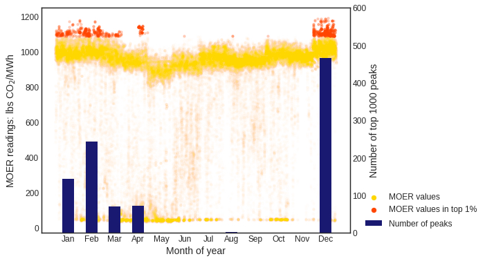
Winter months have the highest marginal emissions

We analyze peak MOER periods, i.e., the 1000 time periods (\(\sim 1\%\) of 5-minute time periods in a year) with the highest MOER values over 2018. Figure 2 illustrates the MOER over the course of 2018, alongside a count of the number of peak MOER periods in each month. The winter and spring months (December through April) account for most of them, which has implications for load shed: shedding loads during the winter months can have the highest impact on emissions.

Figure 2.Scatter plot of MOER values across 2018 highlighting the peak MOER periods, overlaid by a bar plot indicating the number of peak MOER periods in each month.

Some time periods have a sharp drop-off in marginal emissions intensity within an hour

The MOER differential characterizes the emissions reduction possible if one unit of energy consumption can be shifted, i.e., consumed at another time up to one hour before or after its original consumption time. Figure 3 illustrates how prioritizing load shift actions at peak MOER differential times will have a much higher impact on emissions than at other time periods. MOER differentials exhibit a trend by time of day, and most of the high MOER differential time periods lie between 6 am - 6 pm. This has implications for load shift: shifting loads that are active during this window will lead to the highest emissions reductions. The short drop-off period in MOER indicates that is critical to accurately forecast MOER, since even a small window of error could result shifting load to a high MOER period.

Figure 3.On the left, the spread of MOER differentials over the course of 2018 arranged in descending order, overlaid by a plot of potential emissions reduction if load is shifted for an increasing share of time periods over the year.

In the middle, the MOER differential values by hour of day, with the top 1% highlighted in orange. On the right, the spread of MOER differentials in the PJM market region in May 2023 arranged in descending order.

The PJM marginal emissions data also exhibits a similar drop-off in the MOER differentials, albeit with a higher magnitude. This is because even a small change in energy consumption can affect the distribution of power outputs across a range of marginal generators. For example, an increase of 1 MWh in demand at a particular node in the power network could cause the operator to increase output from a fossil fuel powered generator by 500 MWh, and decrease output from a wind farm by 499 MWh, depending on the power network congestion patterns (PJM 2022). Due to data accessibility constraints, we are only able to analyze marginal emissions intensity in the month of May 2023 from the PJM territory. However, the use of additional data from a market operator validates our observation that there are particular times of the year when the MOER differential is particularly high.

End-use loads that are active during high emissions periods

The top end-use loads active during peak MOER periods (ref. Table 2) are plug loads and heating, which makes them a good target for load shed measures. Out of the shiftable end-use loads, the top ones active during peak MOER differential periods are plug loads and refrigeration (ref. Table 2), which makes them a good target for load shift measures. Since load only needs to be shifted over a few time periods, fast discharge batteries can be good candidates to enable this load shift.