Loading [Contrib]/a11y/accessibility-menu.js
Findings
  • Menu
  • Articles
    • Resilience Findings
    • Transport Findings
    • Urban Findings
    • All
  • For Authors
  • Editorial Board
  • About
  • Blog
  • search

    Sorry, something went wrong. Please try your search again.
    ×

    • Articles
    • Blog posts

RSS Feed

Enter the URL below into your favorite RSS reader.

https://findingspress.org/feed
×
Transport Findings
May 08, 2019 AEST

Predicting Response Rates of All and Recruited Respondents: A First Attempt

Basil Schmid, Kay W. Axhausen,
predicting measurement rating stated choice experiments response burden response rate
Copyright Logoccby-nc-4.0 • https://doi.org/10.32866/7827
Photo by Bing HAO on Unsplash
Findings
Schmid, Basil, and Kay W. Axhausen. 2019. “Predicting Response Rates of All and Recruited Respondents: A First Attempt.” Findings, May. https://doi.org/10.32866/7827.
Save article as...▾
  • PDF
  • XML
  • Citation (BibTeX)
Data Sets/Files (5)
Download all (5)
  • Table 1: Response Burden: Points by Question Type and Action
    Download
  • Table 2: Base Populations, Sample Sizes, Ex-ante Assessment of Response Burden, and Response Rates for 68 Survey Wavesa,b
    Download
  • Table 3: Logistic Regression Results: Response Rates 1 (R1; all) and 2 (R2; committed)
    Download
  • Figure 1: R1 and Ex-ante Assessment of Response Burden
    Download
  • Figure 2: R2 of the Committed and Ex-ante Assessment of Response Burden
    Download

Sorry, something went wrong. Please try again.

If this problem reoccurs, please contact Scholastica Support

Error message:

undefined
×

View more stats

Abstract

This paper reports on the link between a well-defined measure of response burden and response rates among all (uncommitted) and pre-recruited respondents. We show within the limits of our sample of 68 survey waves (including pre-tests; resulting from 35 studies) that the response burden impact is mediated by the level of the commitment of the respondents and the presence of a monetary incentive. This is the first time that a research group provides a response rate forecasting model for its own work and for others to adopt, test and adapt.

RESEARCH QUESTION AND HYPOTHESES

When conducting mailback surveys, academics and market researchers must estimate response rates in advance in order to predict the total expected usable responses resulting from a number of mailed questionnaires (and hence to budget their study). Our hypothesis is that, ceteris paribus, the response rate will be inversely proportional to the survey response burden, the level of commitment of the respondents, and the presence of a monetary incentive. Our work is, to our knowledge, the first to quantify this link for the response burden of an instrument, and therefore the first to enable the survey designer to trade off the burden against the response of a survey.

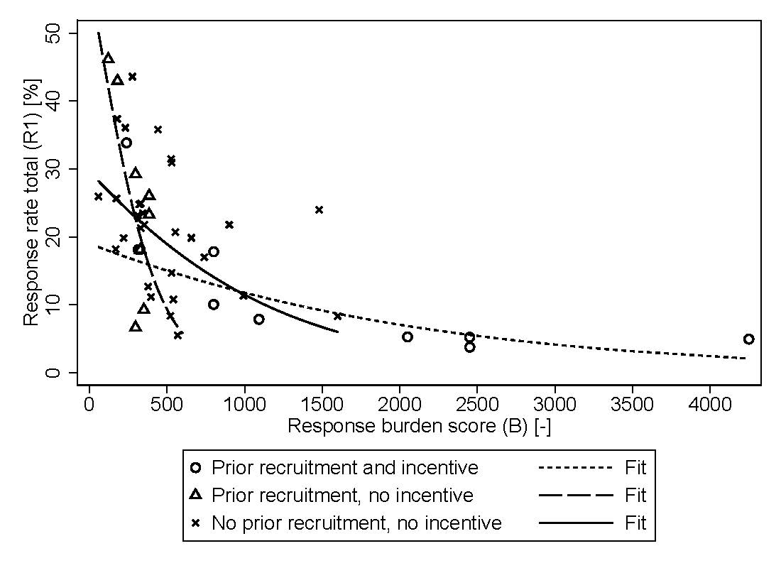
We report results for two types of response rates: Response rate of the share of responses among the total sample (R1) (using the American Association for Public Opinion Research [2016] definition) and response rate of the recruited/committed respondents completing the survey among those who had explicitly agreed to participate (R2).

There is little literature to help in predicting the response burden and corresponding response behavior. There is a large body of literature discussing response rates, the factors influencing them, and the various impacts on survey quality. While the literature on survey methods for paper-based instruments discusses response burden, it does not measure it in detail (see Richardson, Ampt, & Meyburg, 1995; Dillman, Smyth, and Christian, 2014 for relevant textbooks; or the Transportation Research Board wiki). Response burden approximated as the number of pages (or questionnaire length) has a significant influence on the response rate (see also a similar measure in Bruvold and Comer, 1988). Later reviews find the same effect, but do not measure the burden in detail (see Edwards et al., 2002). Current literature on web-based instruments is equally large, but again it misses an a priori measure of the response burden. Bartel-Sheehan (2006), in her review of email questionnaires, finds a clear effect from the number of questions, but does not differentiate by question complexity.

METHODS AND DATA

The response burden (B) is measured with the scheme in Table 1, question by question in an efficient and reproducible way, also accounting for the type and complexity of questions (Axhausen, Schmid, and Weis 2015). Points are added up, such that longer and/or more complex instruments exhibit higher total response burden scores (see also Table 2). Note that twelve points roughly correspond to a one-minute response time (Schmid, Balac, and Axhausen 2018).

Table 1:Response Burden: Points by Question Type and Action
Item Points
Question or transition (up to 3 lines) 2
Each additional line 1
Closed yes/no answers 1
Simple numerical answer (e.g., year of birth) 1
Rating with up to 5 possibilities 2
Rating with more than 5 possibilities 3
Left, middle, right rating 2
Scales with 3 and more grades 2
Best of ranking with cards 4
Second and each additional best ranking 3
Answer to sub-questions of up to 5 words 1
Answers to sub-question of up to 2 lines 2
a) Response to half-open question with ≤8 possibilities 2
Each additional one 2
b) Response to half-open question with ≥8 possibilities 4
Each additional one 3
Answer to “please specify” 2
First answer to an open question 6
Each additional answer to the open question 3
Mixing showcards 6
Giving/showing a card to the respondent 1
Per response category on a showcard 1
Filter 0.5
Branching 0.5
For each stated choice question with 2 alternatives 2
For each stated choice question with 3 alternatives 3
For each variable of the stated choice situation and each question 1

Table adapted from Gesellschaft für Sozialforschung (GfS), Zürich, 2006. First published in Axhausen & Weis, 2010.

The original point system is used to budget face-to-face interviews at the Zürich-based Gesellschaft für Sozialforschung. Ursula Raymann (GfS, Zürich) and later the authors rated the self-administered surveys (Table 2) of the Institute for Transport Planning and Systems (IVT). The current available sample of 68 survey waves including pre-tests (resulting from 35 studies) allows us to test and quantify the stated hypotheses.

Table 2:Base Populations, Sample Sizes, Ex-ante Assessment of Response Burden, and Response Rates for 68 Survey Wavesa,b
Content of the self-administered
surveys / year of study
Location /
base population
Sample sizec Response burden
(old)
Response burden
(updated)
Response rated (%) Cooperation ratee (%)
No prior recruitment With recruitment
No motivation call Motivation call No incentive With incentive
N = 22 N = 8 N = 19 N = 19
1. National SP survey on railway services (2004) Residents of French- and German-speaking part of Switzerland 1,561 84 120 67.7 43.9
2. Regional mode and route choice SP (2006) Residents of Canton Zürich 1,229 84 120 70.9
3. National SP on value of travel time savings (2007) Residents of Switzerland 2,317 153 303 52.7
4. Regional SR on value of statistical life (2004) Residents of Canton Ticino 500 197 440 41.0
5. Regional SR on value of statistical life (2006) Residents of German-speaking part of Switzerland 2,000 224 526 33.9
6. Home ownership and use of local facilities (2005) Residents in a quota sample of municipalities in the Zürich region 9,330 231 36.1
7. National SP on the impacts of road pricing (2007) Residents of French- and German-speaking part of Switzerland 2,249 265 524 46.7
8. Mobility biographies and regular travel behavior (2005) Residents of Cantons Basel, Bern, and Zürich 3,500 521 8.4
9. Mobility biographies (2005) Residents of Canton Zürich 1,763 + 1,537 529 14.7 30.9 21.7
10. Mobility biographies and home ownership (2005) Residents of Canton Zürich 300 655 19.9
11. Social networks and mobility biographies (2006) Residents of Canton Zürich 4,200 992 11.3
12. Mobility plan: University of Zürich (2008) Employees of the university 372 219 19.8
13. Mobility plan: Zürich University Hospital (2008) Visitors to the hospital 1,615 57 25.9
14. Fuel price and rail usage (2009) Residents of Switzerland 1,036 170 327 58.3 18.1
15. Modelling mountaineers’ travel behavior (2009) Members of the Swiss Alpine Club 530 276 46.0
16. Ego-centric social networks: network questionnaire (2009) Residents of Canton Zürich 761 + 91 900 21.8 67.3 23.7
17. Ego-centric social networks: diary (2009) Residents of Canton Zürich 50 + 142 1,480 24.0 57.0
18. Induced traffic (pen-and-paper; 2010) Residents of Canton Zürich 200 800 50.5 24.0
19. Induced traffic (online; 2010) Residents of Canton Zürich 140 800 40.7 14.3
20. 2000 Watt society (pre-test 1: 2010) Residents of Canton Zürich 51 326 76.5 11.3
21. 2000 Watt society (pre-test 2; 2010) Residents of Canton Zürich 49 314 79.6 18.1
22. 2000 Watt society, main study (2010) Residents of Canton Zürich 491 238 80.2 33.8
23. ARE SP (pre-test, mode choice only; 2010) Residents of Switzerland 99 235 68.7
24. ARE SP (pre-test, route choice only; 2010) Residents of Switzerland 29 280 58.6
25. ARE SP (pre-test, mode and route choice; 2010) Residents of Switzerland 484 384 71.9 32.4
26. ARE SP (main study, mode choice only; 2010) Residents of Switzerland 893 235 69.4
27. ARE SP (main study, route choice only; 2010) Residents of Switzerland 215 280 66.5
28. ARE SP (main study, mode and route choice; 2010) Residents of Switzerland 3,994 384 69.3 30.3
29. Residential choice (Otte, no addresses; 2011) Residents of Canton Zürich 1,238 320 24.8
30. Residential choice (Otte, with addresses; 2011) Residents of Canton Zürich 1,238 330 21.3
31. Residential choice (own items, no addresses; 2011) Residents of Canton Zürich 1,239 344 23.5
32. Residential choice (own items, with addresses; 2011) Residents of Canton Zürich 1,238 354 21.8
33. Grimsel user SP (2011) Users of the Grimsel pass 399 180 71.4 43.0
34. Survey on bus and tram use (2011) Residents of Cantons Bern, Lucerne, and Zürich 3,300 310 23.2
35. Survey on parking behavior (2011) Residents of French- and German-speaking part of Switzerland 1,243 404 83.9
36. Survey on travel time reliability (2012) Residents of French- and German-speaking part of Switzerland 491 400 72.7
37. Social behavior in evacuation scenarios (2011) Residents of French- and German-speaking part of Switzerland 4,049 330 24.9
38. Mobility Biographies (2013) Residents of Dortmund (Germany) 336 1,600 8.3
39. Potential of carpooling (2012) Employees from the French- and German-speaking part of Switzerland 1,683 350 52.1 16.2
40. Value of time and reliability (pen-and-paper; 2012) Residents of Germany 3,355 600 64.9
41. Value of time and reliability (online; 2012) Residents of Germany 209 600 54.5
42. Value of time and reliability (commercial; 2012) Residents of Germany 925 500 90.9
43. Climate change influence on Swiss transportf (interviews; 2012) Swiss public and private stakeholders in energy, tourism, and transport sectors 16 48 38.0 37.5
44. Climate change influence on Swiss transportg (pen-and-paper; 2013) Swiss public and private stakeholders in energy, tourism, and transport sectors 5 165 80.0
45. Climate change influence on Swiss transport (online; 2014) Swiss public and private stakeholders in energy, tourism, and transport sectors 55 168 18.0
46. Free-floating car sharing: mobility pilot study (2014) Mobility customers in Canton Basle 2,224 173 25.7
47. Free-floating car sharing: mobility pilot study (2014) Catch-a-car customers in Canton Basle 527 178 37.4
48. Social networks and travel behavior (2014) Residents of Switzerland 208 580 51.4
49. Work location choice (pre-test; 2015) Residents of German-speaking part of Switzerland 265 290 69.4
50. Work location choice (cold calling; 2015) Residents of German-speaking part of Switzerland 11 296 90.9 7.3
51. Work location choice (postal invitation; 2015) Residents of German-speaking part of Switzerland 140 296 83.6 31.8
52. ARE SP 2015 (all waves; 2015) Residents of Switzerland 6,099 296 76.9
53. Travel behavior in a post-car worldh (pre-test; 2015) Households of Canton Zürich 67 4,250 52.2 4.9
54. Travel behavior in a post-car worldh (wave 1; 2015) Households of Canton Zürich 133 2,450 54.1 5.1
55. Travel behavior in a post-car worldh (wave 2; 2015) Households of Canton Zürich 191 2,450 60.2 3.8
56. Travel behavior in a post-car worldh (wave 3; 2016) Households of Canton Zürich 118 2,050 63.6 5.3
57. Social networks and mobility behavior (survey 1; pre-test; 2017) Residents of Canton Zürich 500 740 17.0
58. Social networks and mobility behavior (survey 2; pre-test; 2017) Residents of Canton Zürich 57 470 89.5
59. Social networks and mobility behavior (survey 1; main survey; 2017) Residents of Canton Zürich 12,000 553 20.7
60. Social networks and mobility behavior (survey 2; main survey; 2017) Residents of Canton Zürich 1,706 1,588 81.4 55.8
61. Automated vehicles survey (2017) Residents of Canton Zürich 482 1,092 62.2 7.9
62. SVI: influence of soft factors on travel behavior (pre-test, movers, online, and pen-and-paper; 2018) Residents of German-speaking part of Switzerland 241 540 10.8
63. SVI: influence of soft factors on travel behavior (pre-test, non-movers, online, and pen-and-paper; 2018) Residents of German-speaking part of Switzerland 252 378 12.7
64. SVI: influence of soft factors on travel behavior (main survey, movers, online, and pen-and-paper; 2018) Residents of German-speaking part of Switzerland 4,825 568 5.5
65. SVI: influence of soft factors on travel behavior (main survey, non-movers, online, and pen-and-paper; 2018) Residents of German-speaking part of Switzerland 4,601 396 11.5

Sources: 1. Vrtic & Axhausen, 2004; 2. Vrtic & Fröhlich, 2006; 3. Axhausen et al., 2007; 4. Locatelli, 2004; 5. Jäggle, 2006; 6. Waldner et al., 2005; 7. Vrtic et al., 2007; 8. Schiffmann, 2005; 9. Beige, 2006 and Beige & Axhausen, 2006; 10. Beige, 2004; 11. Axhausen, Frei, & Ohnmacht, 2006; 12. Weis et al., 2008; 13. Weis et al., 2008; 14. Weis & Axhausen, 2009; 15. Stäubli, 2009; 16. Kowald et al., 2009i; 17. Kowald et al., 2009i; 18. Weis et al., 2010; 19. Weis et al., 2010; 20. Jäggi & Axhausen, 2010; 21. Jäggi & Axhausen, 2010; 22. Jäggi & Axhausen, 2010; 23. Fröhlich et al., 2012; 24. Fröhlich et al., 2012; 25. Fröhlich et al., 2012; 26. Fröhlich et al., 2012; 27. Fröhlich et al., 2012; 28. Fröhlich et al., 2012; 29. Schirmer, Belart, & Axhausen, 2011; 30. Schirmer, Belart, & Axhausen, 2011; 31. Schirmer, Belart, & Axhausen, 2011; 32. Schirmer, Belart, & Axhausen, 2011; 33. Steinle, 2011; 34. Scherer, 2011; 35. Weis et al., 2012; 36. Lu, 2014; 37. Kowald et al., 2012; 38. Ehreke & Axhausen, 2015; 39. Mühlethaler et al., 2011; 40. Axhausen et al., 2014; 41. Axhausen et al., 2014; 42. Axhausen et al., 2014; 43. Bösch & Ciari, 2014; 44. Bösch & Ciari, 2014; 45. Bösch & Ciari, 2014; 46. Becker & Axhausen, 2017; 47. Becker & Axhausen, 2017; 48. Rau, 2014; 49. Hirzel, 2015; 50. Hirzel, 2015; 51. Hirzel, 2015; 52. Weis et al., 2017; 53. Schmid, Balac, & Axhausen, 2018; 54. Schmid, Balac, & Axhausen, 2018; 55. Schmid, Balac, & Axhausen, 2018; 56. Schmid, Balac, & Axhausen, 2018; 57. Guidon et al., 2017; 58. Guidon et al., 2017; 59. Guidon et al., 2017; 60. Guidon et al., 2017; 61. Becker & Axhausen, 2018; 62. Schmid et al., (forthcomingj); 63. Schmid et al., (forthcomingj); 64. Schmid et al., (forthcomingj); 65. Schmid et al., (forthcomingj)

aResulting from 35 studies.
bEach survey wave/pre-test counts as a separate observation.
cSample size = total number of potential respondents (i.e., those that received the questionnaires).
dThe numbers correspond to the COOP4 cooperation rate as defined by the American Association for Public Opinion Research (AAPOR, 2016). It is calculated as the number of returned questionnaires, divided by the difference of the total sample size and sample loss (deaths, wrong address, respondent moved).
eOnly reported in case of surveys with prior recruitment and if the numbers were available in the field report. Note that in many surveys with prior recruitment, the total number of respondents who actually received the invitation was not available, leading to a reduced R1 sample size.
f,gObservations are excluded in subsequent analysis because of low total sample size.
hMotivation calls were also conducted.
iNote that the study by Kowald et al. (2009) involved a monetary incentive, phone contact with the interviewers, and a personal post card from a member of the social network to which the respondents belong, inviting them to participate in the survey.
jNo field report/paper available yet.

The following logistic regression model is estimated for the three groups (“no prior recruitment, no incentive”, “prior recruitment, no incentive” and “prior recruitment and incentive”, denoted by subscript i) including weights to capture the number of potential respondents (i.e., who received the questionnaires) in each survey wave and controlling for a global time trend (Y; starting at zero for the year 2004) in response behavior:

\[\mathrm{\log}\left( \frac{\text{R}_{i}}{100 - \text{R}_{i}} \right) = \alpha_{i} + \beta_{i} \ \frac{\text{B}}{1000} + \tau \ Y + \varepsilon_{i}\]

The Logit transformation e.g., (Winkelmann 2006) is applied to the response rate (R) mainly to solve the boundedness problem of the dependent variable (i.e., the probability of participation in a survey; see also Schmid, Balac & Axhausen, 2018). Clustered standard errors are calculated at the study level e.g., (Baltagi 2008).

FINDINGS

The results confirm our hypotheses for both types of response rates. Table 3 shows the results of the logistic regressions (see also Figure 1 and Figure 2). A pooled model for R1 is added for comparison; for an increase in response burden (B) by 100 points, the expected decrease in the odds of participating in a survey is given by \(\left( \exp\left( \frac{\beta_{i}}{1000} \right) - 1 \right)*100\) = 6.0% (p < 0.01). Furthermore, decreasing the age of the study by one year is decreasing the expected odds by 6.8% (p <.05), indicating a general trend of a lower willingness to participate in surveys.

Table 3:Logistic Regression Results: Response Rates 1 (R1; all) and 2 (R2; committed)
Response rate 1 (R1) Response rate 2 (R2)
Variable Pooled model No recruitment, no incentive Prior recruitment, no incentive Prior recruitment and incentive With incentive No incentive
Beta Sig. Beta Sig. Beta Sig. Beta Sig. Beta Sig. Beta Sig.
Constant -0.46 * 0.33 -0.99 ** 0.65 ** 0.77 ***
Constant no, no -0.68 ***
Constant yes, no -0.74 ***
Constant yes, yes -0.75 ***
Response burden (B) -0.60 *** -1.14 *** -4.06 ** -0.48 *** -0.48 *** -2.07 ***
Time trend (Y) -0.07 ** - -0.06 * - 0.09 ***
N 47 29 8 10 19 18
AIC 83.9 - 81.6 a - 60.7a
AICc b 85.3 - 84.5 a - 62.6 a
R2 0.55 - 0.61 a - 0.17 a
Log likelihood (LL) model -36.9 - -33.8 a - -25.3 a
LL intercept(s) only -49.5 - -49.5 a - -32.4a
McFadden R2 c 0.25 - 0.32 a - 0.22a
Significance levels: * = 10%; ** = 5%; *** = 1%

aGoodness-of-fit measures reported for model with different intercept and slope coefficients.

bAIC: The Akaike Information Criterion stands for the relative quality of a model for a given set of observations and can be used to compare different modelling approaches. A smaller AIC means a better fit. AICc is for finite sample size corrected AIC and penalizes larger models more than AIC does.

cMcFadden R2 = 1 – LL (model) / LL (constant only)

Figure 1
Figure 1:R1 and Ex-ante Assessment of Response Burden

Note: Fitted values result from a model without time trend for better readability.

Figure 2
Figure 2:R2 of the Committed and Ex-ante Assessment of Response Burden

Note: Fitted values result from a model without time trend for better readability.

The effect of the response burden in the pooled model averages across the three groups but hides the substantial differences shown in the case-specific analysis. Importantly, an AICc comparison indicates that the fit of the full model (different slope coefficients) is slightly better. While the number of observations is too small to obtain confident statements for all categories, the patterns are clear. The lower share of respondents, those who begin a “cold-call” survey, are then committed to it, and the effect of the response burden is comparable to the respondents which were recruited and offered an incentive. The pattern for the recruited respondents without incentives is reversed: A higher share of respondents start, but there is a dramatic drop in response with an increasing response burden. It should be noted that the incentives were offered for high response burden surveys to overcome this hurdle in recruitment. The results for R2 confirm that the effect of the recruitment is not strong enough to balance the response burden.

To further validate these results, they would need to be replicated by other research groups with the studies available to them. We will continue to expand our sample, but the IVT group will never have enough studies to be confident about the generality of our estimates and we are tied to our social context and subject area with its specific saliency to the respondents (Groves, Presser, and Dipko 2004). Nevertheless, as a first guess the results should allow designers elsewhere to trade-off survey burden versus response and should improve the budgeting substantially.

ACKNOWLEDGMENTS

The authors are very grateful for the rating of the first set of surveys by Ursula Raymann, GfS Zürich, and for making the initial rating scheme available to us.

The article builds on Axhausen and Weis (2010) and Axhausen, Schmid, & Weis (2015).

References

American Association for Public Opinion Research. 2016. Standard Definitions: Final Dispositions of Case Codes and Outcome Rates for Surveys. 9th ed. AAPOR.
Google Scholar
Axhausen, K.W., I. Ehreke, A. Glemser, S. Hess, C. Joedden, K. Nagel, A. Sauer, and C. Weis. 2014. “Ermittlung von Bewertungsansätzen Für Reisezeiten Und Zuverlässigkeit Auf Basis Der Schätzung Eines Modells Für Modale Verlagerungen Im Nicht-Gewerblichen Und Gewerblichen Personenverkehr Für Die Bundesverkehrswegeplanung, FE-Projekt 96.996/2011 Zeitkosten Personenverkehr, Bericht an Das Bundesministerium Für Verkehr Und Digitale Infrastruktur (BMVI).” Berlin.
Axhausen, K.W., A. Frei, and T. Ohnmacht. 2006. “Networks, Biographies and Travel: First Empirical and Methodological Results.” In The 11th International Conference on Travel Behaviour Research (IATBR 2006). Kyoto, August.
Google Scholar
Axhausen, K.W., S. Hess, A. König, G. Abay, M. Bierlaire, and J.J. Bates. 2007. “State of the Art Estimates of the Swiss Value of Travel Time Savings.” In The 68th Annual Meeting of the Transportation Research Board. Washington, D.C., January.
Google Scholar
Axhausen, K.W., B. Schmid, and C. Weis. 2015. “Predicting Response Rates Updated, Arbeitsberichte Verkehrs- Und Raumplanung, 1063.” IVT, ETH Zürich, Zürich.
Axhausen, K.W., and C. Weis. 2010. “Predicting Response Rate: A Natural Experiment.” Survey Practice 3.
Google Scholar
Baltagi, B. 2008. Econometric Analysis of Panel Data. New York: John Wiley and Sons.
Google Scholar
Bartel-Sheehan, K.B. 2006. “E-Mail Survey Response Rates: A Review.” Journal of Computer-Mediated Communication 6.
Google Scholar
Becker, F., and K.W. Axhausen. 2017. “Predicting the Use of Automated Vehicles.” In The 17th Swiss Transport Research Conference. Ascona, May.
Google Scholar
Becker, H., and K.W. Axhausen. 2018. “Analyse Des Angebots von Catch a Car in Basel.” In Arbeitsberichte Verkehrs- Und Raumplanung, 1380. IVT, ETH Zürich, Zürich.
Google Scholar
Beige, S. 2004. “Ownership of Mobility Tools in Switzerland.” In 4th Swiss Transport Research Conference (STRC 2004). Ascona, March.
Google Scholar
———. 2006. “Long-Term Mobility Decisions during the Life Course.” In The 6th Swiss Transport Research Conference (STRC 2006). Ascona, March.
Google Scholar
Beige, S., and K.W. Axhausen. 2006. “Long-Term Mobility Decisions during the Life Course: Experiences with a Retrospective Survey.” In The 11th International Conference on Travel Behaviour Research (IATBR 2006). Kyoto, August.
Google Scholar
Bösch, P.M., and F. Ciari. 2014. “Climate Change Influence on Swiss Transport, Tourism and Energy - A Stakeholders Perspective.” In The 14th Swiss Transport Research Conference (STRC 2014). Ascona, May.
Google Scholar
Bruvold, N.T., and J.M. Comer. 1988. “A Model for Estimating the Reponse Rate to a Mailed Survey.” Journal of Business Research 16: 101–16.
Google Scholar
Dillman, D.A., J.D. Smyth, and L.M. Christian. 2014. Internet, Phone, Mail, and Mixed-Mode Surveys: The Tailored Design Method. English edition. New York: John Wiley and Sons.
Google Scholar
Edwards, P., I. Roberts, M. Clarke, C. DiGuiseppi, S. Pratap, R. Wentz, and I. Kwan. 2002. “Increasing Response Rates to Postal Questionnaires: Systematic Review.” BMJ 324: 1183–92.
Google Scholar
Ehreke, I., and K.W. Axhausen. 2015. “Modellierung von Arbeitsplatzentscheidungen in Mobilitätsbiographien.” In Räumliche Mobilität Und Lebenslauf - Studien Zu Mobilitätsbiografien Und Mobilitätssozialisation, edited by C. Holz-Rau and J. Scheiner, 261–76. Wiesbaden: Springer.
Google Scholar
Fröhlich, P., K.W. Axhausen, M. Vrtic, C. Weis, and A. Erath. 2012. “SP-Befragung 2010 Zum Verkehrsverhalten Im Personenverkehr.” Research Report. Federal Office for Spatial Development (ARE), ETH Zürich, Zürich.
Groves, R.M., S. Presser, and S. Dipko. 2004. “The Role of Topic Interest in Survey Participation Decisions.” Public Opinion Quarterly 68: 2–31.
Google Scholar
Guidon, S., M. Wicki, K.W. Axhausen, and T. Bernauer. 2017. “Investigating the Relationship between Individuals’ Social Networks, Mobility Behaviour and Social Capital - Survey Methods and First Results.” In The 17th Swiss Transport Research Conference (STRC 2017). Ascona, May.
Google Scholar
Hirzel, N. 2015. “Wie Wichtig Ist Die Fahrt Zum Arbeitsplatz?” Eine stated preference Befragung, MSc thesis, IVT, ETH Zürich, Zürich.
Jäggi, B., and K.W. Axhausen. 2010. “Surveying Energy Efficiency in Housing and Transport Using a Priority Evaluator.” Arbeitsberichte Verkehrs- und Raumplanung, 636, IVT, ETH Zürich, Zürich.
Jäggle, B. 2006. “Was Ist Den Schweizern Ein Verhinderter Verkehrstoter Wert?” MSc Thesis, Vienna: Universität für Bodenkultur.
Kowald, M., C. Dobler, and K.W. Axhausen. 2012. “Soziales Verhalten in Grossräumigen Evakuierungsereignissen: Ergebnisse Einer Expertenbefragung.” Arbeitsberichte Verkehrs- und Raumplanung, 710, IVT, ETH Zürich, Zürich.
Kowald, M., A. Frei, J.K. Hackney, J. Illenberger, and K.W. Axhausen. 2009. “The Influence of Social Contacts on Leisure Travel: A Snowball Sample of Personal Networks.” In The 12th International Conference on Travel Behaviour Research (IATBR 2009). Jaipur, December.
Google Scholar
Locatelli, G. 2006. “Valuation of a Statistical Life Saved: Experimental Results from the Ticino, MSc.” Thesis, Milan: Politecnico di Milano.
Lu, M. 2014. “RP and SP Data-Based Travel Time Reliability Analysis.” PhD dissertation, ETH Zürich, Zürich.
Mühlethaler, F., K.W. Axhausen, F. Ciari, M. Tschannen-Süess, and U. Gertsch-Jossi. 2011. “Potenzial von Fahrgemeinschaften.” Schriftenreihe, 1371, UVEK, Bern.
Google Scholar
Rau, U. 2014. Verkehrsverhalten Und Soziale Netzwerke. Masterarbeit, IVT: ETH Zürich, Zürich.
Google Scholar
Richardson, A.J., E.S. Ampt, and A.H. Meyburg. 1995. Survey Methods for Transport Planning. Melbourne: Eucalyptus Press.
Google Scholar
Scherer, M. 2010. “Tram or Bus: Who Preferers What and Why? Stated Reasons for Preference.” Arbeitsberichte Verkehrs- und Raumplanung, IVT, ETH Zürich, Zürich.
Schiffmann, S. 2005. “Mobilitätsbiographie: Verkehrserzeugung Im Alltag.” MSc thesis, IVT, ETH Zürich, Zürich.
Schirmer, P., B.C. Belart, and K.W. Axhausen. 2011. “Location Choice in the Greater Zürich Area - An Intermediate Report.” In The 11th Swiss Transport Research Conference (STRC 2011). Ascona, May.
Google Scholar
Schmid, B., M. Balac, and K. W. Axhausen. 2018. “Post-Car World: Data Collection Methods and Response Behavior in a Multi-Stage Travel Survey.” Transportation 46 (2): 425–92. https://doi.org/10.1007/s11116-018-9968-2.
Google Scholar
Stäubli, A. 2009. “Matterhorn Retour - Modellierung Des Mobilitätsverhaltens von Alpinisten.” Term paper, IVT, ETH Zürich, Zürich.
Transportation Research Board wiki. n.d. Accessed April 16, 2019. http://www.travelsurveymanual.org/.
Vrtic, M., and K.W. Axhausen. 2004. “Forecast Based on Different Data Types: A before and after Study.” In The 10th World Conference on Transport Research (WCTR 2004). Istanbul, July.
Google Scholar
Vrtic, M., and P. Fröhlich. 2006. “Was Beeinflusst Die Wahl Der Verkehrsmittel?” Der Nahverkehr 24: 52–57.
Google Scholar
Vrtic, M., N. Schüssler, A. Erath, and K.W. Axhausen. 2007. “Route, Mode and Departure Time Choice Behaviour in the Presence of Mobility Pricing.” In The 86th Annual Meeting of the Transportation Research Board. Washington, D.C., January.
Google Scholar
Waldner, U., M. Löchl, M. Bürgle, and K.W. Axhausen. 2005. “Haushaltsbefragung Zur Wohnsituation Im Grossraum Zürich - Feldbericht.” Arbeitsberichte Polyprojekt Zukunft urbane Kulturlandschaften, 1, NSL, ETH Zürich, Zürich.
Weis, C., and K.W. Axhausen. 2009. “Benzinpreis Und Bahnnutzung, Report to Swiss National Railways.” IVT, ETH Zürich, Zürich.
Weis, C., C. Dobler, and K.W. Axhausen. 2010. “Stated Adaptation Survey of Activity Scheduling Reactions to Changing Travel Conditions: Field Work and Preliminary Results.” In The 12th World Conference on Transport Research (WCTR 2010). Lisbon, July.
Google Scholar
Weis, C., A. Frei, K.W. Axhausen, T. Haupt, and B. Fell. 2008. “A Comparative Study of Web- and Paper-Based Travel Behaviour Surveys.” In The European Transport Conference. Noordwijkerhout, September.
Google Scholar
Weis, C., M. Vrtic, B. Schmid, and K.W. Axhausen. 2017. “Analyse Der SP Befragung 2015 Zur Verkehrsmodus- Und Routenwahl.” Research Report to the Federal Office for Spatial Development (ARE), IVT, ETH Zürich, Zürich.
Weis, C., M. Vrtic, P. Widmer, and K.W. Axhausen. 2012. “Influence of Parking on Location and Mode Choice: A Stated Choice Survey.” In The 91st Annual Meeting of the Transportation Research Board. Washington, D.C., January.
Google Scholar
Winkelmann, R. 2006. Analysis of Microdata. Berlin: Springer.
Google Scholar

Powered by Scholastica, the modern academic journal management system