Online Large-Scale Taxi Assignment: Optimization and Learning

Omar Rifki; Thierry Garaix

doi:10.32866/001c.74765

Rifki, Omar, and Thierry Garaix. 2023. “Online Large-Scale Taxi Assignment: Optimization and Learning.” Findings, May. https://doi.org/10.32866/001c.74765.

Download all (4)

Figure 1. An example of taxi path building on a $2G$ graph.
Download
Table 1. Results of simulation by varying $\#taxis$ , $T^{request}_ {max}$ , and $T^{reop}$ .
Download
Figure 2. Average number of optimizations in one time step (#opt).
Download
Figure 3. Architecture of the RNN.
Download

View more stats

Abstract

We propose a solution method for online vehicle routing, which integrates a machine learning routine to improve tours’ quality. Our optimization model is based on the Bertsimas et al. (2019) re-optimization approach. Two separate routines are developed. The first one uses a neural network to produce realistic pick-up times for the customers to serve. The second one relies on Q-learning in addition to random walks for the construction of the backbone graph corresponding to the instance problem of each time step. The second routine gives improved results compared to the original approach.

1. Questions

More optimization solvers opt for machine learning (ML) integration in order to take advantage of pattern recognition in the search for solutions (Bengio, Lodi, and Prouvost 2021; Karimi-Mamaghan et al. 2022). Online optimization^[1] poses several challenges for this integration to happen, such as the change of the problem structure across the optimization periods, plus the duration of the period or the time step, which could be very short to perform learning. In online vehicle routing problems (Jaillet and Wagner 2008), this issue can happen for instance, in case the vehicles’ locations and the customers’ requests are revealed over time. We study the online taxi problem as defined by Bertsimas, Jaillet, and Martin (2019), where the transportation requests issued from customers are revealed a number of minutes before their pick-up time and their assignment to taxis has to be acknowledged within minutes before. This is a special case of the online vehicle routing problem (see Appendix A for a formal definition). Their approach manages to solve the online taxi problem for a large demand: about 600-6500 customers for each re-optimization which lasts 30 seconds in the area of Manhattan. It offers then a good starting point to test the optimization-ML integration in a dynamic context. Our basic idea is to design ML routines within the re-optimization in order to improve the quality of the constructed tours. We show that learning can happen even in the case of tight time steps.

2. Methods

The re-optimization of Bertsimas, Jaillet, and Martin (2019) relies on a great simplification of the working graph of the problem with the aim to make the resolution more tractable for each time step. The formal problem definition and their proposed approach are presented in Appendix A. The first ML routine that we implemented is based on the neural network structure. Because of its poor results, this method is only detailed in Appendix B.

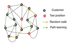
Our second ML routine uses reinforcement learning on the working graph to construct the paths of taxis, in addition to using random paths. This routine replaces steps 2 through 7 of Algorithm 1 (see Appendix A), with random paths and paths constructed with the Q-learning algorithm (Watkins and Dayan 1992) on the $KG$ graph^[2]. Both types of paths start from the current positions of the taxis, as shown in the example of Figure 1. Once a total of $E_{max}$ arcs are chosen from $KG$ , the MIPmaxflow is solved on this constructed graph. This procedure is done iteratively. Learning for each agent taxi is performed across the different iterations of MIPmaxflow within one time step through Q-learning. The main parameter of the routine is the percentage $p_{rl} \in [0,1]$ of taxis that construct their paths using learning. These agents are chosen from all taxis in the first iteration in a random way, as follows:

perform random walks starting from all taxis,
solve MIPmaxflow for this selection, and
choose the $p_{rl}\times 100$ taxis which have the largest rewards,

Figure 1.An example of taxi path building on a

$2G$ graph.

By this way, we can concentrate learning on the seemingly most favorable taxis. Random walks are taken to be non-backtracking in this routine. The description of the steps of the routine is shown in Algorithm 1. As you may notice, no solving of maxFlow is performed. The state space of Q-learning represents the set of nodes of $G$ : $\mathcal{S}=V$ . The current state of each agent taxi is its current node. If a given agent taxi is in a vertex with no outgoing neighbor, it stops exploring, otherwise, it chooses a neighbor according to the Q-table. All the agents explore their neighborhoods in a sequential way. The reward of each agent taxi is given at the end of each iteration in step number 10, by the reward computed for each taxi from the MIPmaxflow resolution. Thus, the reward of each agent taxi depends on the choices of the remaining agents. Setting a state space $\mathcal{S}=V^T$ , where each agent accounts for all other agents’ current positions is time-consuming. Thus, we did not account for it, given the limited time allowed for optimization in a time step.

Algorithm 1.Q-learning routine

Input: The graph

$G$ , the parameter

$K$ , a starting solution

$s$ , and the probability of agent taxis

$p_{rl}$ .

Output: A solution for the current time step

1: while time is available do

2: First iteration: Fix the agent taxis

$T$ using

$p_{rl}$ ;

3: Initialize the backbone graph

$BG$ by removing all arcs

$KG;$

4: Add solution s to

$BG;$

5: while

$BG$ has less than

$E_{\max} \times \left( 1 - p_{rl} \right)$ arcs do

6: For each taxi

$t$ not in

$T$ , generate a random walk on

$KG$ from

$t$ ;

7: Add those arcs to

$BG;$

8: end while

9: All agents choose their actions (paths) using Q-learning to complete

$E_{\max}$ arcs in

$BG;$

10: Solve MIPmaxflow on

$BG;$

11: Update the solution

$s;$

$12:$ end while

Concerning the implementation of the Q-learning policy, we use Monte Carlo methods to estimate the state-action value. For the exploration strategy, we use the epsilon-greedy method with a parameter $\epsilon = 0.1$ .

For comparison matters, we consider the case with only random walks $p_{rl}=0$ , denoted RW-based routine.

3. Findings

Results of Table 1 rely on the Bertsimas, Jaillet, and Martin (2019) dataset, which is based on the demand for taxis on the Manhattan network^[3]. More details on the construction of the dataset and the implementation are provided in Appendix C. We set the simulation time to 20 minutes, and $E_{max}=2000$ . The maximum request times $T_{max}^{request}$ , the number of taxis #taxis, and the time step $T^{reop}$ are varied as in the table below. For each customer $c$ , the request time $t_{c}^{request}$ is uniformly picked within the interval $[t_c^{min}-T_{max}^{request}, t_c^{min}]$ . The time allowed for re-optimization in each time step is equal to the half of $T^{reop}$ , meaning that if $T^{reop}=5min$ , only $2.5min$ is allowed to construct the solution, the remaining time is reserved to transfer the new actions to the taxis. We fix $p_{rl}=10\%$ . In the table, #nser designates the number of not served customers in each simulation.

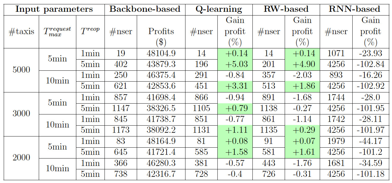
Table 1.Results of simulation by varying

$\#taxis$ ,

$T^{request}_ {max}$ , and

$T^{reop}$ .

These results show that Q-learning subroutine approach offers higher gaps of profits than the RNN routine, surpassing Bertsimas, Jaillet, and Martin (2019) approach in the following cases: i/ when the re-optimization time step is larger than 1min, but can be still considered small (5min), and ii/ when the supply of transport is large compared to the demand (5000 taxis). The explanation behind the changes of #nser in function of #taxi, $T_{max}^{request}$ and $T^{reop}$ is given in Appendix D. The data of Manhattan taxi requests are characterized by a large traffic demand and a large supply of taxis. Any improvement of only $1\%$ of the profit gains can be translated into thousands of US dollars over the day. Compared to the random walks subroutine, the Q-learning subroutine produces higher profit gaps, suggesting that the effect of reinforcement learning is mostly positive. Figure 2 displays the average number of optimizations in a time step for the four approaches.

Figure 2.Average number of optimizations in one time step (#opt).

ACKNOWLEDGMENTS

We would like to thank unknown referees for their comments. This research was funded by the project FITS -“Flexible and Intelligent Transportation Systems” (ANR-18-CE22-0014) operated by the French National Research Agency (ANR).

Submitted: January 27, 2023 AEST

Accepted: April 25, 2023 AEST

References

Alom, Md Zahangir, Tarek M. Taha, Chris Yakopcic, Stefan Westberg, Paheding Sidike, Mst Shamima Nasrin, Mahmudul Hasan, Brian C. Van Essen, Abdul A. S. Awwal, and Vijayan K. Asari. 2019. “A State-of-the-Art Survey on Deep Learning Theory and Architectures.” Electronics 8 (3): 292. https://doi.org/10.3390/electronics8030292.

Google Scholar

Bengio, Yoshua, Andrea Lodi, and Antoine Prouvost. 2021. “Machine Learning for Combinatorial Optimization: A Methodological Tour d’horizon.” European Journal of Operational Research 290 (2): 405–21. https://doi.org/10.1016/j.ejor.2020.07.063.

Google Scholar

Bertsimas, Dimitris, Patrick Jaillet, and Sébastien Martin. 2019. “Online Vehicle Routing: The Edge of Optimization in Large-Scale Applications.” Operations Research 67 (1): 143–62. https://doi.org/10.1287/opre.2018.1763.

Google Scholar

Innes, Mike. 2018. “Flux: Elegant Machine Learning with Julia.” Journal of Open Source Software 3 (25): 602. https://doi.org/10.21105/joss.00602.

Google Scholar

Jaillet, Patrick, and Michael R. Wagner. 2008. “Online Vehicle Routing Problems: A Survey.” Operations Research/Computer Science Interfaces, 221–37. https://doi.org/10.1007/978-0-387-77778-8_10.

Google Scholar

Karimi-Mamaghan, Maryam, Mehrdad Mohammadi, Patrick Meyer, Amir Mohammad Karimi-Mamaghan, and El-Ghazali Talbi. 2022. “Machine Learning at the Service of Meta-Heuristics for Solving Combinatorial Optimization Problems: A State-of-the-Art.” European Journal of Operational Research 296 (2): 393–422. https://doi.org/10.1016/j.ejor.2021.04.032.

Google Scholar

Tian, Jun. 2020. “ReinforcementLearning.Jl: A Reinforcement Learning Package for the Julia Programming Language.” 2020. https://github.com/JuliaReinforcementLearning/ReinforcementLearning.jl.

Watkins, Christopher J.C.H., and Peter Dayan. 1992. Machine Learning 8 (3/4): 279–92. https://doi.org/10.1023/a:1022676722315.

Google Scholar

Supplementary Materials

A. Supplementary materials: Model

The taxi problem is a special case of the dial-a-ride problems, where vehicles are allowed to serve only one customer at a time. In the online context, each customer $c \in \mathcal{C}$ has a request time $t_c^{request}$ , a confirmation time $t_c^{conf} > t_c^{request}$ , when the optimizer confirms to $c$ whether his request is accepted or not, and a pick-up time window $I_c=[t_c^{min}, t_c^{max}]$ .

Bertsimas, Jaillet, and Martin (2019) model the problem as a directed graph $G (V,E)$ where the nodes represent the customers $c \in \mathcal{C}$ and the current positions of the taxis $k \in \mathcal{K}$ . Each arc $(c',c)$ has an associated profit $R_{c', c}$ , which is equal to the fare paid by the customer $c$ to satisfy minus the cost of driving from the drop-off point of $c'$ , or from the position of the taxi in case of arc $(k, c)$ and $c$ is the first customer visited by the taxi $k$ . The main assumption of the model is that the working graph $G$ has no cycle. This is made possible by deleting arcs that do not satisfy the time windows of the customers in addition to other tighter time constraints. It is important to notice that the shorter the time windows are, the fewer cycles exist in $G$ . The objective of the optimization is to maximize the total profit of the solution. Without sub-tours elimination, the routing problem becomes a network max-flow problem, with integer and real-valued variables. The mixed integer programming formulation of the offline problem, i.e. $t_c^{request} = 0, \forall c \in \mathcal{C}$ , is as follows.

$\max_{x,y,p_c, t_c} \quad \sum_{k \in \mathcal{K}, c \in \mathcal{C}}{R_{k, c}y_{k, c}}+\sum_{c, c' \in \mathcal{C}}{R_{c', c}x_{c', c}} \tag{1}$

$\text{s.t.} \quad p_c = \sum_{k \in \mathcal{K}} y_{k, c} \ \ \ \ \ \ \ \ \ \ \forall c \in \mathcal{C} \tag{2}$

$\sum_{c \in \mathcal{C}}x_{c', c} \leq p_{c'} \ \ \ \ \ \ \ \ \ \ \forall c' \in \mathcal{C} \tag{3}$

$\sum_{c \in \mathcal{C}}y_{k, c} \leq 1 \ \ \ \ \ \ \ \ \ \ \forall k \in \mathcal{K} \tag{4}$

$x_{c',c}\in \{0,1\} \ \ \ \ \ \ \ \ \ \ \forall c', c \in \mathcal{C} \tag{5}$

$y_{k,c}\in \{0,1\} \ \ \ \ \ \ \ \ \ \ \forall k \in \mathcal{K}, \forall c \in \mathcal{C} \tag{6}$

$p_c \in \{0,1\} \ \ \ \ \ \ \ \ \ \ \forall c \in \mathcal{C} \tag{7}$

$t_c^{min} \leq t_c \leq t_c^{max} \ \ \ \ \ \ \ \ \ \ \forall c \in \mathcal{C} \tag{8}$

$\small{ t_c \geq t_c'+(t_c^{min}-t_{c'}^{max}) + (T_{c',c}-(t_c^{min}-t_{c'}^{max})) x_{c',c}\; \ \ \ \ \ \ \ \ \ \ \forall c', c \in \mathcal{C} \tag{9} }$

$t_c \geq t_c^{min} + (t_k^{init}+T_{k,c}-t_c^{min})y_{k,c} \ \ \ \ \ \ \ \forall k \in \mathcal{K}, \forall c \in \mathcal{C} \tag{10}$

$T_{c',c}$ designates the travel time to serve $c'$ and to drive to the pick-up location of $c$ . The decision variables $y_{k,c}$ and $x_{c,c'}$ specify the order of visit of the customers for each taxi, while $p_c$ tells if customer $c$ is served or not, and $t_c$ provides the pick-up time of $c$ . This problem is denoted MIPmaxFlow. When the customers’ pick-up times are fixed, the max-flow problem, i.e. (1)-(7), becomes efficiently solvable through the simplex algorithm, thanks to some integrality results (see Theorem 1. of Bertsimas, Jaillet, and Martin (2019). We denote this subproblem maxFlow.

The approach of Bertsimas, Jaillet, and Martin (2019) to solve the online version consists of solving MIPmaxFlow in each time step for customers with known request times, or in other terms with $t_c^{request} \leq k T^{reopt}$ , such that $T^{reopt}$ is the time step duration, and $k T^{reopt}$ corresponds to the starting time of the current re-optimization. To scale the optimization to the real-world high demands scenario, the authors adopt the routine described in Algorithm 2. At first, the graph $G$ containing the current customers and the current taxi positions is pruned into a graph $KG$ , by selecting the $K$ best incoming and outgoing arcs of each node of $G$ in terms of lost times, which are defined as waiting times plus times of a taxi driving empty. Then, a backbone graph $BG$ is constructed iteratively by solving maxFlow problem on uniformly generated pick-up times, before solving MIPmaxflow on the constructed graph. This step is done repeatedly. The parameters $E_{max}$ and $K$ are chosen such that MIPmaxflow and maxFlow are solvable in reasonable times. More complete details of the model and the algorithm choices are found in Bertsimas, Jaillet, and Martin (2019).

Algorithm 2.Backbone-based routine

Input: The graph

$G$ , the parameter

$K$ , the limit number

$E_{\text{max~}}$ , and a starting solution

$s$ (could be empty)

Output: A solution for the current time step

1: Compute

$KG$ ;

2: while time is available do

3: Initialize the backbone graph

$BG$ by removing all arcs of

$KG;$

4: while

$BG$ has less than

$E_{\max}$ arcs do

5: For each customer

$c$ , generate uniformly a pick-up time

$t_{c}$ from

$I_{c}$ or from

$I_{c}^{s}$ (is the time window where the solution

$s$ is propagated in

$I_{c}$ );

6: Solve maxFlow on

$KG$ with the

$t_{c}$ pick-up times of the customers;

7: Add the optimal arcs of the solution to the graph

$BG;$

8: end while

9: Solve MIPmaxflow on

$BG;$

10: Update the solution

$s;$

11: end while

B. Supplementary materials: RNN routine

This ML routine has the goal to learn the most adequate pick-up times of the customers, and then solve maxFlow problem for these times. We choose the Recurrent Neural Network (RNN) for the architecture, which is a neural network well suited to manage vector sequences over time (Alom et al. 2019).

The routine replaces steps 3 to 10 of Algorithm 2. Instead of randomly generating pick-up times (step 5) and solving the maxFlow problem for these times (step 6) for the construction of the support backbone graph (stage 7), we learn the pick-up times of the customers and solve maxFlow problem for these optimal times. No solving of MIPmaxflow is involved. The description of the steps is shown in Algorithm 3. The obtained solution updates the current solution similarly to Algorithm 2.

Algorithm 3.RNN-based routine

Input: The graph

$G$ , the parameter

$K$ , and a starting solution

$s$ (could be empty)

Output: A solution for the current time step

1: Compute

$KG;$

2: while time is available do

3: while exploration time is available do

4: For each customer

$c$ , generate uniformly a pick-up time

$t_{c} \in I_{c}$ or

$t_{c} \in I_{c}^{s};$

5: Solve maxFlow on

$KG$ with

$t_{c}$ pick-up times of customer;

6: Add the arc profits of the solution to features

$X$ and

$\left( t_{c} \right)$ to

$y;$

7: end while

8: Train the RNN model

$m$ using

$X$ and

$y;$

9: Generate times by

$\left. \ \mathbf{t} = m\left( \left\lbrack R_{e_{1}},\ldots,R_{|E|} \right) \right\rbrack^{'} \right);$

10: Solve maxFlow with times

$\mathbf{t};$

11: Update the solution

$s;$

12: end while

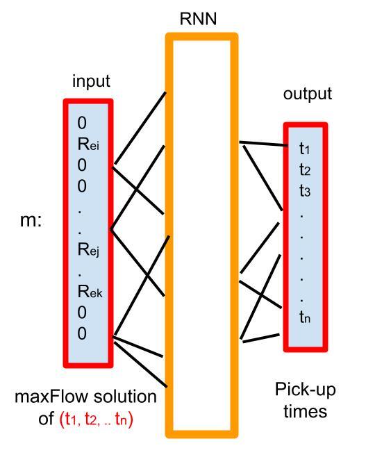
For the training of the RNN, we solve maxFlow with pick-up times uniformly chosen at random within customers’ time windows. We also include in the training the times corresponding to the upper bounds of the time windows. The RNN outputs the customers’ pick-up times and takes for inputs the solution of the corresponding maxFlow problem, which is in our case a vector over the graph arcs such that if an arc belongs to the solution, its profit value ( $R_{c',c}$ or $R_{k,c}$ ) is taken, otherwise zero. A scheme of RNN is shown in Figure 3. We obtain the learned pick-up times of the current re-optimization by taking as input the profits of all the arcs of the graph $KG$ . Regarding the RNN architecture, we use the sigmoid activation function, plus the cross entropy loss function and the Adam optimizer. According to our tests, tuning across other RNN hyperparameters does not improve the result of the RNN routine. We set the exploration time here (the step 3 of Algorithm 3) to two third of the time allowed for optimization in each time step.

Figure 3.Architecture of the RNN.

C. Supplementary materials: Data

The data consists of several elements. The first element is the demands of the customers, which come from the taxi-trip dataset of the New York City Taxi and Limousine Commission on the area of the Manhattan network. It is constructed by filtering requests with pick-up and drop-off points located in Manhattan. For each customer, $t_c^{min}$ is set to the real pick-up time, $t_c^{max} = t_c^{min} + 5min$ , and $t_c^{conf} = t_c^{min}-4min$ . The request time $t_c^{request}$ is a variable of the simulation. Bertsimas, Jaillet, and Martin (2019) use the demands of Yellow Cabs alone on a specific day, which is 04/15/2016. We use the same inputs.

The second element is the travel times in the Manhattan network. Bertsimas, Jaillet, and Martin (2019) use the Yellow Cabs data to estimate those times. Having no access to this data, we set travel times according to OpenStreetMap (OSM) in the following way. For each road segment, we set the speed to the maximum speed given by OSM. In the following step for the simplification of the network, if two or more segments are merged, we set the speed to the minimum of the merged segments’ speeds. This allows us to considerably reduce the speed in the network since taking the maximum speed is not a reasonable assumption. The shortest path computation uses travel times computed using those speeds. For the profit computation, we use the customer’s real fare set with costs taken proportional to the trip travel times: a cost of 5$ per hour of driving and a cost of 1$ per hour of waiting, same as Bertsimas, Jaillet, and Martin (2019).

The approaches that are compared in Table 1 share the same input data for each simulation run : the same travel times and request times $t_c^{request}$ . In order to run Bertsimas, Jaillet, and Martin (2019)'s program, we convert their Julia source code from version $0.5$ to a stable version $\geq 1.0$ .

D. Supplementary materials: Demand/supply balance

The quality of the solutions, thus the profits and the number of not served customers, changes according to the number of taxis. With 2000 taxis (and $(T_{max}^{request}, T^{reop})=(5,1)$ ), the solution covers $18\%$ more transportation requests than that of 3000 taxis (and $(T_{max}^{request}, T^{reop})=(5,1)$ ), due to a better-performing arc selection procedure for the backbone graph (steps 4-8 in Algorithm 2; steps 5-9 in Algorithm 1). This is because all problems share the same value of the maximum number of arcs $E_{max}=2000$ . This latter value is taken to make the MIPmaxFlow optimization possible in a short duration. If the number of taxis increases, the selection of arcs is altered. With 5000 taxis, the excess of vehicles makes it possible to correct the lack of coverage with 4000 and 3000 taxis. There is almost always a free taxi able to serve a new customer request. Thus, the solutions’ profits become in the same range of the case of 2000 taxis. Notice that the number of not served customers increases as the time step $T^{reop}$ and/or the maximum request times $T_{max}^{request}$ increase, since more customers are present in MIPmaxFlow optimizations compared to the base case of $(T_{max}^{request}, T^{reop})=(5,1)$ .

Online optimization is a field of optimization theory for which the input data of the problem are revealed over time and decisions have to be given in between.
A pruned graph of the working graph of the problem $G$ (see Appendix A for a definition of $KG$ , MIPmaxflow and maxFlow problems).
The Julia libraries Flux.jl (Innes 2018) and ReinforcementLearning.jl (Tian 2020) are used for the implementation.