1. Questions
Finding fast and efficient solutions has been a hot topic in post-disruption restoration problems. Although some studies attempted to find realistic network restoration planning models (Bienstock and Mattia 2007; Nurre and Sharkey 2014; Nan and Sansavini 2017; Ermagun and Tajik 2021), they never incorporated the effects of routing time on the network performance trajectory after disruptions. Other studies developed models to capture the routing time restoration crews across the network (Özdamar, Tüzün Aksu, and Ergüneş 2014; Kasaei and Salman 2016; Akbari and Salman 2017; Faturechi and Miller-Hooks 2014; Iloglu and Albert 2018; Ermagun and Tajik 2022). Due to the complex nature of routing problems discussed by Morshedlou et al. (2021), new models are designed to calculate efficient bounds for real-world problems. This research proposes a time-dependent restoration scheduling problem to produce a feasible and efficient initial solution to address the following questions: How does the spatial distribution of disruptions affect the complexity of the problem? Does partially activating under restoration links affect the network resilience trajectory?
2. Methods
The model illustrates the network performance as the total flow on an undirected graph \(G = (N,A),\) where \(N\) is the set of nodes, and \(A\) is the set of links. Among the nodes, there is a set of origin nodes \(N_{+} \subseteq N,\) each with capacity \(O_{i},\ i \in N_{+},\) a set of destination nodes \(N_{-} \subseteq N,\) each with a demand requirement \(b_{i},\ i \in N_{-},\) and a set of transshipment nodes \(N_{=} \subseteq N.\) Each link \((i,j) \in A,\) has a capacity of \(u_{ijt_{e}}\) at time \(t_{e}\) before disruptions. After disruptions, a subset \(A' \subseteq A\) represents the set of disrupted links, each with a new capacity \(u_{ijt_{d}} < u_{ijt_{e}}.\) The model deploys crews to restore disrupted locations in the residual network in a critically limited time horizon. Only one crew is permitted to restore a disrupted location. Each crew \(k \in K\) can restore each disrupted link \((i,j) \in A^{\prime}\) in \(p_{ij}^{k}\) time units. The main assumption, called Binary Activation, declares that each disrupted link will not return to its operational status unless fully restored. During the restoration process, the model records the routing time of each crew \(k \in K,\) including its traveling time between each pair of consecutives assigned disrupted links \((l,h),(i,j) \in A'\) \(\left( c_{(lh)(ij)} \right).\) The maximum restoration crew routing time must not exceed the given time horizon \(\left( T_{\max} \right).\) The goal is to represent a convenient model, called as Binary Active model, to maximize the residual network resilience \((Я_{\varphi}(t))\) by recovering the critical disrupted links in a given time horizon per Equation 1. The network resilience \((Я_{\varphi}(t))\) measures the network performance as the aggregate difference between the total delivered flow \(\left( \varphi_{it_{d}} \right)\) to destination nodes \(\left( i \in N_{-} \right)\) immediately after disruption at the time \((t_{d})\) and the those of \(\varphi_{it}\) at each time period \((t)\) in the restoration horizon over the difference between total network performance \(\left( \varphi_{it_{e}} \right)\) before disruptions at time \((t_{e})\) and after disruptions \(\left( \varphi_{it_{d}} \right).\)
\[Max\ \sum_{t = 1}^{T_{Max}}{Я_{\varphi}(t)} = \sum_{t = 1}^{T_{Max}}{\sum_{i \in N_{-}}^{\mathstrut}\frac{\varphi_{it} - \varphi_{it_{d}}}{\varphi_{it_{e}} - \varphi_{it_{d}}}}\tag{1}\]
Other variables required for the mathematical model are as follows:
\(\alpha_{kijt}:\) 1: If Crew \(k \in K\) recovers Link \((i,j) \in A^{\prime}\) at Time \(t;\) 0: Otherwise (binary)
\(\vartheta_{d}^{k}:\) 1: If restoration Crew \(k \in K\) originates from Depot \(d \in D;\) 0: Otherwise (binary)
\(\ f_{ijt}:\) Flow on Link \((i,j) \in A'\) in Time period \(t\) (continuous)
\(\complement_{(lh)\ (ij)}^{k}:\) Travel time of Crew \(k \in K\) on the shortest path between Links \((l,h),(i,j) \in A'\) (continuous)
\(\complement_{.\ }^{k}:\) Travel time of Crew \(k \in K\) from its originating depot \((d \in D)\) (continuous)
\(c_{d\ (ij)}:\) Travel time on the shortest path between Depot \(d \in D\) and the disrupted Link \(\left( i,j \right) \in A^{\prime}\) (continuous)
Table 1.Binary Active Formulation
| Equations |
Indexes |
No. |
| \(\sum_{j:(i,j) \in A}^{\mathstrut}f_{ijt}\mathbf{-}\sum_{j:(j,i) \in A}^{\mathstrut}f_{jit} \leq O_{i}\) |
\[\forall i \in N_{+}\ ,\ t = 1,\ldots,T\] |
(2) |
| \(\sum_{j:(i,j) \in A}^{\mathstrut}f_{ijt} - \sum_{j:(j,i) \in A}^{\mathstrut}f_{jit} = 0\) |
\[\forall i \in N_{=}\ ,\ t = 1,\ldots,T\] |
(3) |
| \(\sum_{j:(i,j) \in A}^{\mathstrut}f_{ijt} - \sum_{j:(i,j) \in A}^{\mathstrut}f_{jit} = - \varphi_{it}\) |
\[\forall i \in N_{-}\ ,\ t = 1,\ldots,T\] |
(4) |
| \(0 \leq \varphi_{it} \leq b_{i}\ \) |
\[\forall i \in N_{-}\ ,t = 1,\ldots,T\] |
(5) |
| \(0 \leq f_{ijt} \leq u_{ijt_{e}}\ \ \) |
\[\forall(i,j) \in A,t = 1,\ldots,T\] |
(6) |
| \(0 \leq f_{ijt} \leq \sum_{s = 1}^{t}{\alpha_{kijs}u}_{ijt_{e}}\) |
\[\forall(i,j) \in A^{\prime},\ t = 1,\ldots,T\] |
(7) |
| \(\sum_{s = 1}^{T}\alpha_{ijs} \leq 1\) |
\[\forall(i,j) \in A'\] |
(8) |
| \(\sum_{(i,j) \in A^{\prime}}^{\mathstrut}{\sum_{s = 1}^{min\{ T,t + p_{kij} - 1\}}\alpha_{kijs}} \leq 1\ \) |
\[k \in K,\ t = 1,..,\ T\] |
(9) |
| \(\sum_{t = 1}^{p_{ijk} - 1}\alpha_{kijt} = 0\) |
\[\forall(i,j) \in A^{\prime},\forall k \in K\] |
(10) |
| \(\complement_{(lh)(ij)}^{k} \geq c_{(lh)(ij)}\left( \alpha_{kijt} + \alpha_{klh\left( t + p_{klh} \right)} - 1 \right)\) |
\[\forall(i,j),(l,h) \in A^{\prime},\ k \in K,\ t = 1,\ldots,T - p_{klh}\] |
(11) |
| \(\complement_{(lh)(ij)}^{k} \leq c_{(lh)(ij)}\alpha_{kijt}\) |
\[\forall(i,j),(l,h) \in A^{\prime},\ k \in K,\ t = 1,\ldots,T - p_{ijh}\] |
(12) |
| \(\complement_{(lh)(ij)}^{k} \leq c_{(lh)(ij)}\alpha_{klh\left( t + p_{klh} \right)}\) |
\[\forall(i,j),(l,h) \in A^{\prime},k \in K,\ t = 1,\ldots,T - p_{klh}\] |
(13) |
| \(\complement_{.\ }^{k}\ = \sum_{(i,j) \in A^{\prime}}^{\mathstrut}{\sum_{d \in D}^{\mathstrut}{\vartheta_{d}^{k}c}_{d\ (ij)}\alpha_{kijp_{kij}}}\) |
\[\forall(i,j) \in A^{\prime},\ k \in K\] |
(14) |
| \(\complement_{.\ }^{k} + \sum_{(i,j) \in A^{\prime}}^{\mathstrut}{\sum_{(l,h) \in A^{\prime}}^{\mathstrut}{\complement_{(lh)\ (ij)}^{k} + \sum_{t = 1}^{T}{p_{ij}^{k}\alpha_{kijt}}}} \leq T_{\max{\ \ }}\) |
\[k \in K\] |
(15) |
| \({\vartheta_{d}^{k},\alpha}_{kijt}\ \epsilon\ \{ 0,1\}\) |
\[d \in D,\ \forall(i,j) \in A^{\prime},\ k \in K,\ t = 1,\ldots,T_{\max}\] |
(16) |
| \(f_{ijt} \geq\)0 |
\[\forall(i,j) \in A^{\prime},\ t = 1,\ldots,T_{\max}\] |
(17) |
| \(\complement_{(lh)\ (ij)}^{k} \geq\)0 |
\[\forall(i,j),(l,h) \in A^{\prime},k \in K\] |
(18) |
| \(\complement_{.\ }^{k} \geq\)0 |
\[k \in K\] |
(19) |
| \(T_{\max} \geq\)0 |
|
(20) |
| \(p_{ij}^{k} \geq\)0 |
\[\forall(i,j) \in A^{\prime},k \in K\] |
(21) |
Equations 2-7 are network flow balance constraints that send flow from supply nodes to the demand nodes through transshipment nodes and control the flow over the entire network. Equations 8-10 schedule and deploy \(|K|\) crews to restore the disrupted links. Equations 11-13 record the shortest path traveling time of Crew \(k \in K\) between two consecutive disrupted locations. Equations 14-15 calculate the routing time of each crew and ensures it does not exceed the given time horizon. Finally, Equations 16-21 constrain the decision variables. An alternative to the Binary Active assumption is allowing disrupted links to become partially operational during restoration, also called the Proportional Active assumption. To implement such an assumption, we introduce a binary variable \(\gamma_{kijt}\) to activate disrupted Link \((i,j)\) under restoration by Crew \(k \in K\) proportional to its restoration progress at time \(t.\) Accordingly, we update the model to a new Proportional Active Model to reflect the new assumption as summarized in Table 2.
Table 2.Proportional Active model
| Equations |
Indexes |
No. |
| Equations (2)-(6) from Table 1 |
|
|
| \(f_{ijt} \leq u_{ijt_{d}} + \sum_{k \in K}^{\mathstrut}{{\sum_{s = 1}^{t}\gamma_{kijs}F}_{kij(t - s)}(u_{ijt_{e}} - u_{ijt_{d}})}\) |
\[\forall(i,j) \in A^{\prime},\ t = 1,\ldots,T\] |
(22) |
| \(\sum_{(i,j) \in A^{\prime}}^{\mathstrut}{\sum_{s = \text{max}\{ 1,t - p_{kij} + 1\}}^{t}\gamma_{kijs}} \leq 1\) |
\[\ \forall k \in K,\ t = 1,\ldots,T\] |
(23) |
| \(\sum_{t = {T - p}_{kij} + 1}^{T}\gamma_{kijt} = 0\) |
\[\forall(i,j) \in A^{\prime},\ \ \forall k \in K\] |
(24) |
| \(\complement_{(lh)(ij)}^{k} \geq c_{(lh)\ (ij)}\left( \gamma_{kijs} + \gamma_{klh(s + p_{kij})} - 1 \right)\) |
\(\forall(i,j),(l,h) \in A^{\prime},\forall k \in K\)
\[s = 1,\ldots,T - p_{kij}\] |
(25) |
| \(\complement_{(lh)(ij)}^{k} \leq c_{(lh)\ (ij)}\gamma_{kijs}\) |
\(\forall(i,j),(l,h) \in A^{\prime},\ \forall k \in K\)
\[s = 1,\ldots,T - p_{kij}\] |
(26) |
| \(\complement_{(lh)(ij)}^{k} \leq c_{(lh)\ (ij)}\gamma_{klhs}\) |
\(\forall(i,j),(l,h) \in A^{\prime},\ \forall k \in K\)
\[s = 1,\ldots,T - p_{klh}\] |
(27) |
| \(\complement_{.}^{k}\ = \sum_{(i,j) \in A^{\prime}}^{\mathstrut}{\sum_{d \in D}^{\mathstrut}{\vartheta_{d}^{k}c}_{d\ (ij)}\gamma_{kij1}}\) |
\[\ \forall k \in K\] |
(28) |
| \(\complement_{.}^{k} + \sum_{(i,j) \in A^{\prime}}^{\mathstrut}{\sum_{(l,h) \in A^{\prime}}^{\mathstrut}{\complement_{(lh)\ (ij)}^{k} + \sum_{t = 1}^{T}{p_{ij}^{k}\gamma_{kijt}}}} \leq T_{\max{\ \ }}\ \) |
\[\ \forall k \in K\] |
(29) |
| \(\gamma_{kijt} = \left\{ 0,1 \right\}\) |
\[(i,j) \in A,\ k \in K,t = 1,\ldots,T\] |
(30) |
Equation 22 calculates the restoration progress, and consequently the proportion of operationality, of each disrupted link \((i,j) \in A^{\prime}.\) Equations 22-24 are the counterparts of Equations 8-10, Equations 25-27 are the counterparts of Equations 11-13, and Equations 28-29 are the counterpart of Equations 14-15. Equation 30 constrains the decision variables.
3. Findings
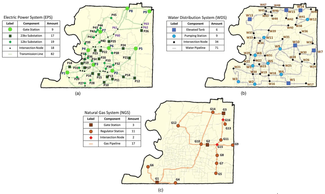
Table 3 shows the computational experiment of the Binary and Proportional active model for gas \((N = 16,A = 17),\) water \((N = 49,A = 71),\) and power grid \((N = 129,A = 164)\) networks in Shelby County, TN (González et al. 2016) as depicted in Figure 1. We incorporate four disruption scenarios \(M = \{ 1,2,3,4\}\) to disrupt incrementally 6%, 9%, 17%, and 23% of the links. Both models calculate the total routing time \((T)\) in presence of \(|K| = 2\) to 7 restoration crews. The results also indicate the computer processing time (CPU), and the optimality gap percentage (GAP). The (-) stands for instances with nonexistent solutions or the ones that require more than one hour of CPU time. The model is implemented using Gurobi Solver 9.0 in Python 3.6.
Table 3.The experimental results
| \[\mathbf{M}\] |
\[\mathbf{|K|}\] |
Network |
| Gas |
Water |
Power |
| Binary |
Proportional |
Binary |
Proportional |
Binary |
Proportional |
| CPU |
Gap (%) |
T |
CPU |
Gap (%) |
T |
CPU |
Gap (%) |
T |
CPU |
Gap (%) |
T |
CPU |
Gap (%) |
T |
CPU |
Gap (%) |
T |
| 1 |
2 |
0 |
0 |
51 |
0 |
0 |
51 |
145 |
0.01 |
144 |
145 |
0 |
132 |
6 |
0.01 |
38 |
11.8 |
0 |
38 |
| 3 |
0 |
0 |
38 |
0 |
0 |
38 |
235 |
0.05 |
88 |
97.1 |
0 |
90 |
6 |
0.24 |
29 |
13.8 |
0 |
36 |
| 4 |
- |
- |
- |
- |
- |
- |
73 |
0.01 |
89 |
144 |
0 |
75 |
7 |
0.03 |
27 |
15.4 |
0 |
26 |
| 5 |
- |
- |
- |
- |
- |
- |
633 |
0.01 |
79 |
123 |
0 |
65 |
8 |
0.05 |
20 |
16.6 |
0 |
23 |
| 6 |
- |
- |
- |
- |
- |
- |
492 |
0.01 |
76 |
200 |
0 |
53 |
- |
- |
- |
- |
- |
- |
| 7 |
- |
- |
- |
- |
- |
- |
384 |
0 |
73 |
240 |
0 |
55 |
1 |
0 |
52 |
8.08 |
6 |
53 |
| 2 |
2 |
0 |
0 |
88 |
8.65 |
0 |
76 |
800 |
0.03 |
189 |
741 |
0 |
224 |
1 |
0 |
39 |
8.70 |
6.90 |
46 |
| 3 |
0 |
0 |
63 |
2.64 |
0 |
74 |
375 |
0.03 |
123 |
504 |
0 |
123 |
1 |
0.01 |
30 |
10.75 |
1.52 |
36 |
| 4 |
0 |
0 |
64 |
3.57 |
0 |
39 |
375 |
0.03 |
123 |
434 |
0 |
95 |
1 |
0.01 |
25 |
13.74 |
6.53 |
30 |
| 5 |
0 |
0 |
56 |
4.47 |
0 |
50 |
771 |
0.02 |
82 |
680 |
0 |
82 |
1 |
0 |
52 |
8.08 |
6 |
53 |
| 6 |
- |
- |
- |
- |
- |
- |
1228 |
0.2 |
80 |
575 |
0 |
74 |
- |
- |
- |
- |
- |
- |
| 7 |
- |
- |
- |
- |
- |
- |
3600 |
5.5 |
79 |
345 |
0 |
67 |
- |
- |
- |
- |
- |
- |
| 3 |
2 |
3 |
0 |
97 |
24.6 |
0 |
100 |
3600 |
2.79 |
272 |
3700 |
9 |
339 |
145 |
0.09 |
60 |
145 |
0.09 |
60 |
| 3 |
2.60 |
0 |
81 |
4.36 |
0 |
74 |
3600 |
0.96 |
177 |
3795 |
3 |
256 |
21 |
0.05 |
45 |
21 |
0.05 |
45 |
| 4 |
3 |
0 |
70 |
4.34 |
0 |
61 |
3600 |
0.96 |
104 |
3700 |
0.6 |
177 |
24 |
0.04 |
38 |
24 |
0.04 |
38 |
| 5 |
2.78 |
0 |
56 |
10.4 |
0 |
54 |
3600 |
0.96 |
102 |
3713 |
0.3 |
140 |
20 |
0.04 |
30 |
20 |
0.04 |
30 |
| 6 |
2.70 |
0 |
46 |
8.78 |
0 |
54 |
3600 |
0 |
79 |
3727 |
0.2 |
124 |
35 |
0.01 |
29 |
35 |
0.01 |
29 |
| 7 |
3 |
0 |
46 |
5.58 |
0 |
61 |
3600 |
2.75 |
65 |
3735 |
0.1 |
106 |
29 |
0.01 |
25 |
29 |
0.01 |
25 |
| 4 |
2 |
3 |
0 |
94 |
13.7 |
0 |
97 |
1624 |
19 |
399 |
3689 |
21 |
402 |
3180 |
1 |
127 |
3180 |
1 |
127 |
| 3 |
3 |
0 |
81 |
5.83 |
0 |
61 |
3600 |
7 |
257 |
3711 |
7 |
276 |
3600 |
0.6 |
91 |
3600 |
0.6 |
91 |
| 4 |
2.80 |
0 |
75 |
5.64 |
0 |
52 |
1624 |
3 |
138 |
3727 |
7 |
251 |
3600 |
0.45 |
69 |
3600 |
0.45 |
69 |
| 5 |
3 |
0 |
65 |
5.22 |
0 |
48 |
1793 |
6 |
106 |
3748 |
1 |
163 |
3600 |
0.3 |
58 |
3600 |
0.3 |
58 |
| 6 |
2.51 |
0 |
56 |
6.24 |
0 |
45 |
3600 |
0 |
81 |
3758 |
0.5 |
146 |
3600 |
0.1 |
51 |
3600 |
0.1 |
51 |
| 7 |
3 |
0 |
50 |
6.69 |
0 |
44 |
3600 |
0 |
75 |
3778 |
0.4 |
126 |
3600 |
0.1 |
48 |
3600 |
0.1 |
48 |
_power_grid_transmission__(b)_wa.png)
Figure 1.Critical infrastructure networks of Shelby County, TN: (a) Power grid transmission, (b) Water, and (c) Gas network (González et al. 2016) The results state a series of empirical observations:
-
The CPU time in Table 3 confirms that the proposed model provides an efficient initial solution for restoration routing problems that assume multiple crews can work on a single disrupted link to expedite its restoration process.
-
Despite their larger network size, the computation processing time and the maximum routing time of power grid instances are less than water network instances. This observation corroborates the importance of the geographical distribution of disruptions, given that the disruptions are scattered across the water network while they are relatively located neighboring one another in the power grid.
-
The proposed model provides a realistic initial solution as it incorporates the routing time of each crew into the restoration scheduling plan. The model optimality gap increases the proportional active feature, reaching high proportional performance earlier than other paths. Although the original model can elevate network performance with a more homogenous rate, the proportional active feature guarantees to restore the spatially distributed disrupted links across a network in a limited time horizon.
Submitted: May 08, 2022 AEST
Accepted: July 29, 2022 AEST