1. Questions
Following the emergence of shared micromobility via scooters and dockless bicycles, several published studies have documented associations between land uses or demographic characteristics and trip generation using these modes. The field has somewhat converged on applying Negative Binomial (“NB”) regression models[1] – a type of count model – or variations of them as the model of choice in studying what factors are associated with trip generation. These models possess several convenient properties for studying trip generation, since trips are countable and often highly concentrated, exhibiting generally nonlinear relationships with urban form.
Unlike in linear regression models, coefficeints of NB regressions and related nonlinear models cannot be interpreted directly as the association between an independent variable and trip counts as would be the case for an Ordinary Least Squares regression: Instead, it is necessary to calculate those associations at specific scenarios (commonly referred to as “marginal effects”; the expected change in trip generation associated with some change in an independent variable from a particular starting point in terms of all variables). Nonetheless, it is common for studies reporting the findings of these models to present model coefficients rather than marginal effects (Bai and Jiao 2020; Gehrke et al. 2021; Huo et al. 2021; Jiao and Bai 2020). To the extent marginal effects are reported at all, they are reported for a single, supposedly representative point in the independent variables’ distributions (Merlin et al. 2021). These forms of reporting mask great heterogeneity across space in the absolute magnitudes of associations, and may not be the most easily interpretable presentation of those relationships, especially in light of actual density distributions across cities.
Urban structure is, of course, highly concentrated and nonlinear: While most of a city’s areal units tend to be of relatively modest densities (in terms of population, or jobs, or amenities), a small handful of tracts – such as central business districts - exhibit supranormal densities. The same nonlinearity and concentration is also true for micromobility trip origination.
Given this, we ask: Do the magnitudes of relationships between land uses and dockless trip generation vary across space within cities? Does this pose a challenge for how to report the findings of an NB regression trip generation model, in particular when trying to make models’ outputs accessible to practitioners?
2. Methods
We demonstrate this effect using a simple land use model of scooter trip generation. Our data consist of 1,142,228 scooter trips undertaken across 408 census blockgroups in Minneapolis, Minnesota between July 10, 2018 and November 26, 2019, as well as independent variables obtained from the 2019 US Census ACS, Census LODES WAC, and OpenStreetMap, all at the census blockgroup level.
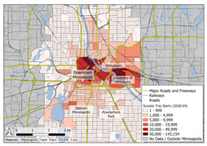
As is demonstrated in Figure 1, scooter trips are highly concentrated Downtown and near the University of Minnesota and decay with distance from those centers, with a smaller concentration of trip origins in the Uptown Minneapolis entertainment district.
Using this data, we model trip generation at the blockgroup level as a function of the variables listed in Table 1: densities of people, jobs, people aged 18-25, and food/drink establishments, as well as of distance from the CBD.[2] The daily average number of trip generations in a block group is the dependent variable, using NB regression.
Finally, we calculate the marginal effect for each independent variable at three different points:[3] At the median in terms of all variables (somewhat resembling a single family home neighborhood), at densities found in blockgroups in Dinkytown and Uptown Minneapolis (major entertainment districts with a large young population), in Powderhorn Park (a medium density urban neighborhood three miles south of Downtown containing a low-rise commercial corridor), and at densities equal to those in the most job-dense blockgroup of Downtown Minneapolis (the regional CBD).
3. Findings
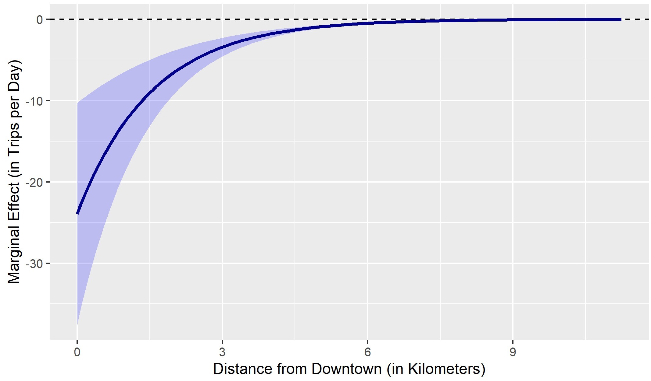
Table 2 presents the regression model as is commonly displayed in the literature, while Table 3 shows marginal effects when using the “starting point” value shown for each independent variable. Table 3 also shows where that starting point is in the distribution of all values in the data. Figure 2 presents marginal effects and confidence intervals for a single variable – distance to downtown – across its entire range, holding all other variables constant at their medians.[4]
As shown in Table 3 and Figure 2, magnitudes of relationships – when expressed as the number of trips per day associated with a one unit change in one of the land use or urban form variables - can vary dramatically across their own range and across different values for other independent variables as a consequence of the mathematical properties of the NB model. This is not immediately obvious from Table 2: Associations are of an economically almost irrelevant magnitude when variables are held at their median, whereas they are very large but statistically insignificant at a starting point resembling a downtown location. Comparing the implied marginal effects between the medians scenario and a scenario resembling the Uptown Minneapolis entertainment district, almost every association differs by approximately one order of magnitude.
The findings from our simple model have several implications for the literature that should be explored, even in models that have a larger set of independent variables: First, relationships between density and trip generation are nonlinear. Secondly and resulting from this first finding, studies using NB or similar models to study trip generation should report associations for several different starting points resembling real-world locations. Doing so would convey information relevant to practitioners – such as the number of incremental scooter trips associated with a particular change in land use – in a more accessible manner, without the risk of misleading by referring to one particular location. Lastly, a property of non-linear models, such as NB, appears to be that the confidence interval around marginal effects grows large near the upper limit of the data. Unfortunately, these are precisely the locations where scooter trips tend to be most common.
Acknowledgements
This research flowed from an earlier research project funded by the METRANS Transportation Consortium. We thank METRANS for funding to support collection of the scooter and some of the land use data used here. Zakhary Mallett was a participant in that earlier research, and we thank him for background research and econometric analysis related to that earlier work.
Some studies also use Zero-inflated Negative Binomial (“ZINB”) regression, a variation of NB that accounts for large numbers of zero outcomes by combining an NB second stage with a logit to model whether or not to expect nonzero outcomes.
The model is purposefully kept simple for demonstration purposes, however, the phenomenon we point out remains with the inclusion of additional dependent variables, or when using ZINB.
Marginal effects are calculated using the “margins” command in Stata.
Differences between the extreme marginal effects in Table 3 for Downtown and Dinkytown and the values shown in Figure 2 as distance approaches zero exist because Figure 2 presents marginal effects for Distance to Downtown with all other variables held at their sample medians, while Table 3 uses values for the specific neighborhoods.


