1. Questions

Accessibility, the ease of reaching destinations, has been proposed as the gold-standard land-use and transport systems performance measure. Accessibility measures are instrumental in assessing the extent to which a land-use and transport system benefits some population groups more than others, thus generating a valuable urban socio-spatial report that can inform planning practice (El-Geneidy and Levinson 2022; Wachs and Kumagai 1973). Although the concept of accessibility has been discussed in academic circles for more than 60 years (Hansen 1959; Handy 2020), planning practitioners still face the challenge of selecting between multiple accessibility measures still debated in academia with no consensus on the horizon. When asked about accessibility measures, practitioners indicated that lack of knowledge and data were their main barriers to adopting accessibility in planning practice (Siddiq and Taylor 2021; Boisjoly and El-Geneidy 2017).

This paper compares two place-based accessibility measures often debated in transport scholarship: gravity-based and cumulative opportunities. Gravity-based accessibility measures have been referred to by some in academic debates as more theoretically sound (as they are not restricted to a single time or distance threshold) and, therefore, superior to the cumulative opportunities approach (Geurs and van Wee 2004; Siddiq and Taylor 2021). By using a distance (or time) decay function inspired by Newtonian physics and observed travel behavior, gravity-based accessibility constructs penalize harder-to-reach destinations more heavily than easier-to-reach ones, continuously, rather than as a binary. However, by weighting opportunities by distance or time, gravity measures also penalize interpretability since the idea of weighted jobs is not easy to grasp in practice, although it can be interpreted as the equivalent number of jobs at your doorstep. In contrast, with cumulative opportunity measures, all destinations reached within a pre-defined travel time (or distance) threshold are weighted equally, and is directly measurable. By having no weights, cumulative opportunity accessibility measures are easier to compute and interpret than gravity-based ones, therefore, more likely to be adopted by planning agencies (El-Geneidy and Levinson 2021; Handy and Niemeier 1997).

Our work draws upon data from Montreal, Canada, and spatial data analytics to answer the following fundamental question: Can easy-to-interpret cumulative opportunity accessibility measures substitute for the more complex-to-calculate and difficult-to-interpret, gravity-based accessibility constructs to improve public transport systems? By answering this question, our paper contributes to the long-standing academic debate on place-based accessibility performance measures and provides empirical-based evidence valuable to land-use planners, transport agencies, and policy-makers.

2. Methods

To compute the accessibility to jobs, we gathered public transport schedules in the General Transit Feed Specification (GTFS) format and for October 2016. A joint network between the public transport network and the streets was then created using the R package r5r developed by Pereira et al. (2021). Then travel times between census tract centroids were computed in r5r based on the joint network during the morning peak hour, on a regular weekday, following Boisjoly and El-Geneidy (2016). To account for travel time variability associated with departure time, we estimated travel times at every minute from 8 AM to 9 AM and reported only the 50th percentile as suggested by Conway et al. (2018). Our commute-by-transit-times estimations in r5r account for walking, waiting, and transfer times.

Jobs data was acquired through Statistics Canada, from the 2016 Census, in the form of commute trips for the Montreal Census Metropolitan Area (CMA). The data set includes the number of commuters working in each Census Tract (CT), their home CT, mode of transport used for the commute, and personal income.^[1] The 30% lowest paying job in the CMA was determined as the city’s low-income threshold – a figure consistent with Deboosere and El-Geneidy (2018) and Foth, Manaugh, and El-Geneidy (2013). According to this threshold, those whose income fell below $30.000 Canadian were classified as having a low-wage job. Others were classified as having a non-low wage job.

Travel times were joined with the commute trip table provided by Statistics Canada to fit multiple travel-time-decay curves and their function parameters. The coefficients of each function were obtained using non-linear least square estimation methods available in the stats R package using the default Gauss-Newton algorithm wrapped into the package’s nls function. Data processing included generating tables with the count of trips by travel time. Net and cumulative commute normalized values were used to generate probability density function (PDF) and inverse cumulative density functions (CDF) based on the number of trips observed at travel times ranging from 1 to 120 minutes.

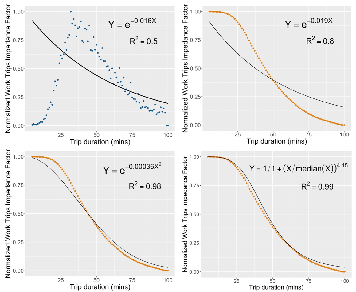
We estimated coefficients for two groups of decay curves. The first group consists of two negative exponential functions (one assuming decay-PDF and another assuming a decay-CDF) and a Gaussian and Log-Logistic decay-CDF (see equations embedded in Figure 1). We also estimated the parameter for a Gaussian and a Log-Logistic decay-CDF decay curve that account for trips and jobs (Levinson and Kumar 1994). More details about our methods are provided in the Supplemental Information section, including equations used to estimate access to employment and coefficient estimates for all decay functions fitted.

Figure 1.Commute-time decay curves and parameters: Negative Exponential PDF (top-left), Negative Exponential CDF (top-right), Gaussian CDF (bottom-left), Log-Logistic CDF (bottom-right)

We estimated cumulative opportunities-based accessibility for each Census Tract for 24 travel time thresholds ranging from 1 to 120 minutes. Then we calculated eight gravity-based measures of accessibility derived from the decay parameters previously estimated and another one assuming a fixed negative exponential decay coefficient of 0.01, which is often used in research when travel behavior data is not available.

Finally, we estimated the Pearson Correlation coefficient between each combination of cumulative and gravity-based accessibility measures. This final step produced a 29 x 29 correlation matrix, from which we answered our research question. We close testing whether the overall trend persists when accounting for differences in income groups and using the first groups of decay functions.

3. Findings

Figure 1 shows commute trips normalized by the maximum observed in the distribution on the y-axis and trip duration on the x-axis. The four curves we fitted are consistent with travel behavior scholarship and will be used derive a subset of gravity-based accessibility measures later in the analysis. Additional information provided in the Supplemental Information Section, Table 1. One remarkable insight from Figure 1 is that the popular negative exponential decay function is the one that distances the most from the distribution of our data and introduces a larger error. A preliminary visual inspection suggests that a Log-Logistic or a Gaussian CDF would provide results more attuned with observed travel behavior as scholars in other disciplines have noted (Deribe, Bauer, and Groneberg 2016). However, a more in-depth analysis indicates that the gravity-based accessibility measures obtained from these four decay curves are strongly correlated (above 0.97). This finding is consistent with empirical evidence presented by Higgins (2019), who used New York City as a case study to estimate walkable accessibility to employment using multiple gravity measures.

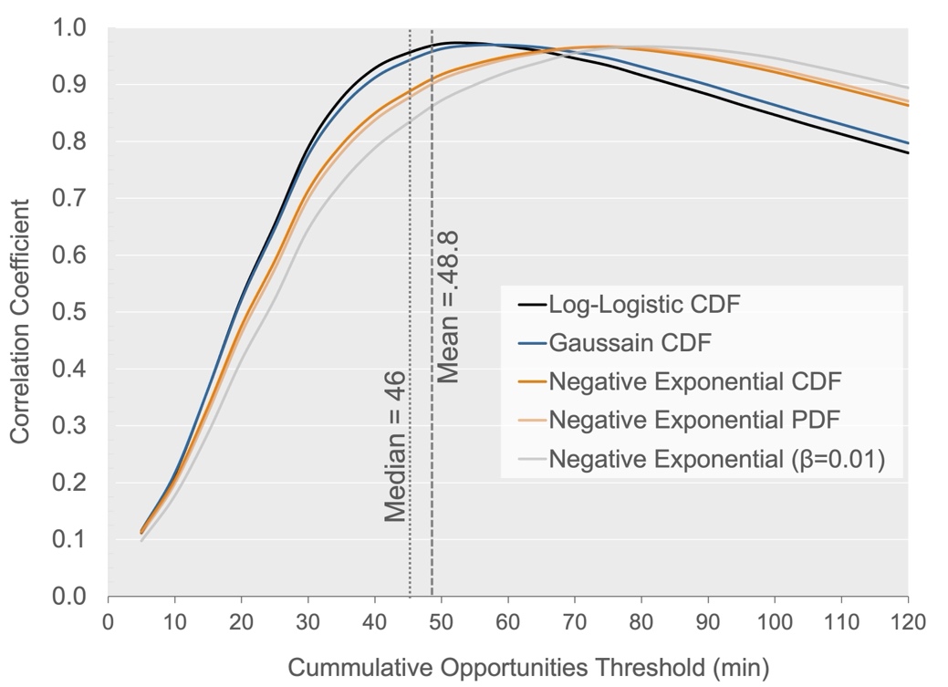
However, this does not mean that gravity-based accessibility measures perform significantly better than parsimonious cumulative opportunities measures. Figure 2 shows how accessibility estimates obtained using the cumulative opportunities approach correlate with accessibility measures estimated using the gravity-based method. To that end, we estimate the Pearson correlation coefficient for each gravity-based measure and cumulative opportunities-based accessibility measures when the latter was assessed at 24 thresholds varying from 5 to 120 minutes (x-axis). We also included the mean and median commute times to have two fixed benchmarks for comparison purposes and provide recommendations.

Figure 2.Correlation between different job accessibility place-based measures Gravity-based accessibily measures derived from decay curves that account for trips

The curves in Figure 2 represent how the correlation between different gravity and cumulative opportunities measures varies for different travel time thresholds. The maximum correlation coefficient (0.97) is reached when the travel time threshold for cumulative opportunities measures is set to the mean commute time of the region (48.8 minutes) with the gravity-based measured derived using Log-Logistic and Gaussian decay CDF. These two decay curves represent observed travel behavior with the minimum error (Figure 1). All correlation coefficients passed our test for statistical significance at a 0.01 confidence level.

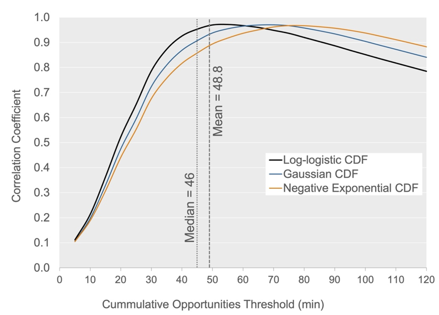
To further demonstrate the stability of the relationship uncovered, we calculated gravity-based accessibility indexes using CDF decay curves that jointly account for observed commute trips and available jobs by time interval (Levinson and Kumar 1994). Coefficient estimates and models’ goodness of fit are provided in the Supplemental Information section, Table 1. Our findings are consistent even after using more complex decay functions accounting for the number of jobs (Figure 3).

Figure 3.Correlation between job accessibility place-based measures. Gravity-based accessibily measures derived from decay curves that account for trips and jobs

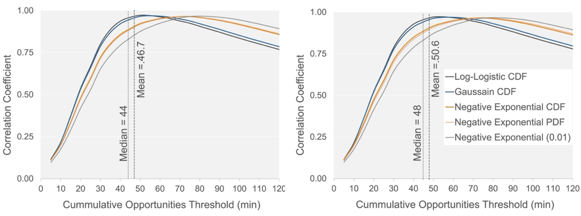
To further demonstrate the observed trend’s stability, we tested the correlation between cumulative opportunities and gravity-based access jobs for low- and non-low-wage jobs.^[2] Figure 4 shows that a correlation coefficient of approximately 0.9 is reached when the threshold to calculate cumulative opportunities accessibility is set to the average commute time for the type of opportunties in question.

Figure 4.Access to low-wage jobs (left) and non-low-wage jobs (right)

Our findings strongly suggest that estimating access to jobs by public transport using the cumulative opportunities approach highly approximates the best performing gravity-based access measures promoted in transport planning and geography scholarship. We hypothesize that such a relationship has to do with the nature of travel time decay functions used since the area under these curves approximate the mean or median commute times in the region – depending on the functional form assumed. This hypothesis can be explored in future research where the mathematical formulation of such relationships can be derived. Our results are robust to income class and other approaches to estimating decay curves that represent travel behavior in the Montreal metropolitan region.

Replicating our work for different urban areas is the next step to confirm such relationships, yet our findings provide a step towards simplifying the adoption of accessibility as a fundamental transport and land-use performance metric in planning practice. Future research should test the validity of the findings with other modes of transport such as walking and cycling, which generally have shorter travel times.

Supplemental Information

For our estimations of accessibility, we used the Hansen (1959) Equation (1) to calculate access to jobs for each census tract in Montreal and derived the language to explain each equation element from Levinson and King (2020)

\[A_{i} = \ \sum_{j}^{}{O_{j}f\left( C_{\text{ij}} \right)}\tag{1}\]

Where:

\(A_{i}:\) access from the centroid of census tract \(i\)
\(O_{j}:\) number of opportunities available at destination \(j\)
\(C_{\text{ij}}:\) cost of travel from \(i\) to \(j\) (travel time)
\(f\left( C_{\text{ij}} \right):\) impedance function

For the case of our cumulative opportunities-based accessibility measures, the impedance function \(f\left( C_{\text{ij}} \right)\) is given by Equation 2, taking a value of one if travel time is less than a threshold \(t\) and zero otherwise.

\[f\left( C_{\text{ij}} \right) = 1\ \text{if}\ C_{\text{ij}} \leq \ t,\ else\ f\left( C_{\text{ij}} \right) = 0\tag{2}\]

And for the case of our gravity-based accessibility measures, impedance factors were estimated following three different functional forms: Negative exponential (Equations 3), Gaussian (Equations 4), and Log-logistic or Fisk (Equation 5).

\[f\left( C_{\text{ij}} \right) = \ e^{\beta\text{\ C}_{\text{ij}}} \tag{3}\]

\[f\left( C_{\text{ij}} \right) = \ e^{{\text{β\ }C_{\text{ij}}}^{2}}\tag{4}\]

\[f\left( C_{\text{ij}} \right) = \ \frac{1}{1 + \left( \frac{C_{\text{ij}}}{\text{median}(C)} \right)^{\beta}}\tag{5}\]

Where:

\(\beta:\) is a decay function coefficient

We derived two groups of decay functions. The first group consisted of commute-time decay functions obtained from a table that classifies trips by commute times using a bin ranging from 5 to 100 minutes, with one-minute increments. From that table, we generated two decay curves. The first consists of a probability distribution curve in which the x-axis represents travel times and the y-axis contain the probability that a trip will take X number of minutes. The likelihood of a trip conducted within each one-minute bin was obtained by dividing the number of trips in each time interval by the total number of trips observed in the region. Then, the obtained probabilities were normalized by dividing each figure by the maximum probability obtained in the previous step. Normalization ensures decay functions generate impedance factors that range from one to zero.

The second consisted of an inverse cumulative probability distribution curve in which the x-axis represents travel times and the y-axis the probability that a trip will take at most X minutes. Such probability was computed by first dividing the number of trips in each time interval, or time band within the bin, by the total number of trips observed in the region and then obtaining the cumulative distribution of those probabilities. Then we normalized each cumulative probabilities value by dividing it by the product of its summation. A final step consisted in obtaining a vector with inverse cumulative probability values calculated as one minus the normalized cumulative value obtained for each travel time interval.

The second group of decay functions was derived from cumulative probability distribution curves that account for trips and jobs, following (Levinson and Kumar 1994), noting that the number of potential destinations increases with travel time from the origin. This estimation method consists of six subsequent steps:

• First, we obtained the total number of trips for all possible combinations of origins and observed travel times, constrained to our 1-minute travel time bin.

• Second, we calculated the number of jobs reached from each origin-time pair.

• The third step consisted of dividing the number of trips by the number of jobs in each origin-time pair.

• In a fourth step, we normalized the ratio of trips to employment in each origin-time bin by dividing such figures by the summation of the ratios across travel times. This latter computation results in a normalized trips-to-jobs ratio for each origin-time pair.

• Then, we obtained the median of the trips-to-jobs normalized ratio in each time interval.

• The sixth and final step consisted in generating a vector with the inverse cumulative probability of the median trips-to-jobs ratio.

Using the data from the two groups of curves generated, we fitted a total of 15 non-linear models to estimate 15 decay function parameters. Model results are shown in Table 1.

Acknowledgments

The authors would like to thank Professors David Levinson at the University of Sydney, Antonio Paez at McMaster University, and Karst Geurs, at University of Twente, for providing feedback on the gravity-based measures calculations. This research was funded by NSERC RGPIN-2018-04501. We would also like to thank Dr. Anson Stewart from Conveyal for helping us troubleshoot how to use their routing engine R5 with the GTFS published by the Société de Transport de Montréal.