Loading [MathJax]/jax/output/SVG/jax.js
Skip to main content
null
Findings
  • Menu
  • Articles
    • Energy Findings
    • Resilience Findings
    • Safety Findings
    • Transport Findings
    • Urban Findings
    • All
  • For Authors
  • Editorial Board
  • About
  • Blog
  • covid-19
  • search

RSS Feed

Enter the URL below into your favorite RSS reader.

http://localhost:25822/feed
Transport Findings
August 21, 2021 AEST

Distributions of Bus Stop Spacings in the United States

Ayush Pandey, Lewis Lehe, Dana Monzer,
public transportationbustransitbus stopstop spacing
Copyright Logoccby-sa-4.0 • https://doi.org/10.32866/001c.27373
Photo by Jay Ee on Unsplash
Findings
Pandey, Ayush, Lewis Lehe, and Dana Monzer. 2021. “Distributions of Bus Stop Spacings in the United States.” Findings, August. https:/​/​doi.org/​10.32866/​001c.27373.
Save article as...▾
Download all (3)
  • Figure 1. Example Transit Network
    Download
  • Figure 2. Traversal-weighted stop spacing distributions
    Download
  • Figure 3. Average Stop Spacing inside and outside core city
    Download

Sorry, something went wrong. Please try again.

If this problem reoccurs, please contact Scholastica Support

Error message:

undefined

View more stats

Abstract

This article introduces a database of bus stop spacings for 43 cities in the United States derived from GTFS files published in late 2019. Weighting each spacing by the number of times a bus traverses it, we produce distributions and summary statistics. The overall mean spacing is 313 meters. Las Vegas’ RTC has the widest mean spacing (482 m) and Philadelphia’s SEPTA the narrowest (214 m). We also compare spacings within agencies’ “core’” cities to those outside.

1. Questions

Bus stop spacing refers to the distance that a bus travels from one stop to the next. Much theoretical analysis has focused on the choice of bus stop spacing (see extensive discussions in Daganzo and Ouyang 2019), which impacts how much time is spent braking and accelerating at stops as well as walking distances. Still, there is little hard data available as to what stop spacings actually are in the United States. One refrain in the literature is that US cities commonly have seven to ten bus stops per mile (Furth and Rahbee 2000; El-Geneidy et al. 2006). The source for this claim can be traced to Reilly (1997, 4), who says “It is common European practice to have stops spaced at 3 or 4 per mile in contrast with 7 to 10 stops per mile, which is common in the United States,” though the study does not cite a particular source for this fact.

This study uses General Transit Feed Specification (GTFS) (Wong 2013) data published by 43 US transit agencies to build a dataset of stop spacings, available at Pandey and Lehe (2021a), in which each row represents one traversal of a spacing. By “traversal” we mean one instance of a bus traveling from one stop to the next stop on the trip. The GTFS files were all published in late 2019—before the service changes wrought by COVID-19. This article introduces the dataset, defines terms and answers some questions using the database:

  1. What are the summary statistics?

  2. How do the distributions of stop spacings look?

  3. How do mean stop spacings differ inside and outside of the “core” cities served by an agency?

2. Methods

2.1. Definitions

We define stop spacing as the distance between two stops along the route of the bus. It includes the distance traveled along any bends in the road.

For distributions and summary statistics of stop spacings, we apply what we call traversal weighting: that is, if the schedule has buses move directly from stop A to stop B 100 times before the schedule repeats, then that spacing is counted 100 times.

To illustrate, consider the simple bus system shown in Figure 1, which shows a network with two routes and three stops. The blue route has two stops spaced 400 m apart and a frequency of 1. The red route has three stops, spaced 200 m apart, and a frequency of 3. The traversal-weighted mean stop spacing for the network in Figure 1 is

400+200⋅3+200⋅31+3⋅2=228.57(m).

If an omnipresent driver were to drive every bus, this is the mean distance he or she would travel between stops on this network.

Figure 1
Figure 1.Example Transit Network

2.2. Calculation

Pereira, Andrade, and Bazzo (2020) introduces an R-package, gtfs2gps, which converts GTFS files to a database in which each row describes the location of a vehicle on a scheduled trip at a point along its route—including at all stops. One piece of data in each row is the cumulative distance that the vehicle has traveled since the start of the current trip. We use this database to produce another database, akin to the one in Table 1, in which each row represents one traversal, giving the distance traveled between the traversal’s two stops and their locations. Example code doing so for Ann Arbor is at Pandey and Lehe (2021b).

Table 1.Representative Database
spacing loc1 loc2
⋮ ⋮ ⋮
xi (lat1,lng1)i (lat2,lng2)i
xi+1 (lat1,lng1)i+1 (lat2,lng2)i+1
⋮ ⋮ ⋮

The general procedure is as follows: First, starting with the initial database produced by gtfs2gps, we filter out all non-bus trips and all rows that do not correspond to a location at a stop, so that the database only contains information about buses when they are at stops. Next, for each stop along each trip, we subtract the cumulative distance traveled (from the start of the trip) when the bus is at the preceding stop from the cumulative distance traveled at the given stop, which gives the distance traveled between the stops. This difference is stored as a row in the new database along with both stops’ coordinates, and the database is made available at Pandey and Lehe (2021a).

3. Findings

We apply the method described in Sec. 2.2 to 43 US cities. The sample includes the six most populated US cities as well as many smaller cities chosen to capture a diversity of city types and regions. The only systematic requirement for inclusion was that a city’s GTFS files be sufficiently “filled in” for gtfs2gps to convert the GTFS files to a GPS database. To run gtfs2gps requires that a GTFS bundle includes certain files: the optional ‘shapes.txt’ file and either the optional ‘frequency.txt’ or certain optional columns in the required ‘stop_times.txt’ file, so it cannot run when agencies do not include some optional data. The particular agency corresponding to each city[1] is listed in Table 2.

Table 2.Summary Statistics (traversal-weighted) for stop spacing (in [m]) in US cities
City Agency Mean Std. Deviation Q25 Median Q75 Core Mean ExCore Mean
Ann Arbor Ann Arbor Area Transportation Authority 383 213 245 325 443 353 438
Bloomington Bloomington Transit 321 199 193 271 387 322 311
Boston Cape Cod Regional Transit Authority 283 206 174 234 323 288 280
Buffalo Niagara Frontier Transportation Authority 262 199 170 218 289 224 328
Charlotte Charlotte Area Transit System 393 282 228 320 455 382 530
Chicago Chicago Transit Authority 223 114 176 205 240 223 236
Cincinnati Southwest Ohio Regional Transit Authority 279 210 167 237 320 265 329
Cleveland Greater Cleveland Regional Transit Authority 275 185 188 243 317 263 289
Columbus Central Ohio Transit Authority 369 229 240 317 420 357 423
Dallas Dallas Area Rapid Transit 300 250 176 242 342 283 372
Denver Regional Transportation District,America/Denver 408 275 261 353 451 373 433
Des Moines Des Moines Area Regional Transit Authority 273 188 177 227 305 247 445
Detroit Detroit Department of Transportation 258 159 182 222 292 245 363
El Paso Sun Metro 415 342 232 312 459 413 497
Fresno Fresno Public Transportation (FAX) 392 220 264 358 450 389 413
Gainesville Regional Transit System 263 122 185 231 295 263 NA
Houston Metropolitan Transit Authority of Harris County 306 187 198 256 357 300 378
Indianapolis Indianapolis Public Transportation Corporation 333 233 196 264 389 331 356
Jacksonville Jacksonville Transportation Authority 450 387 245 341 497 448 520
Kansas City Kansas City Area Transportation Authority 355 278 199 273 411 329 437
Los Angeles Los Angeles County Metropolitan Transportation Authority 402 294 243 341 434 392 418
Las Vegas Regional Transportation Commission of Southern Nevada 482 225 362 425 529 462 491
Memphis Memphis Area Transit Authority 280 246 147 214 328 278 408
Miami Miami-Dade Transit 349 297 192 260 388 288 372
Milwaukee Milwaukee County Transit System 278 175 185 232 354 269 299
Minneapolis Metro Transit 279 212 192 209 300 261 292
New York Metropolitan Transportation Authority Bus Company 328 283 178 240 353 327 448
Oakland AC Transit 344 236 207 283 400 306 371
Omaha Metro Transit 246 149 172 213 275 246 394
Orlando Central Florida Regional Transit Authority 401 290 231 325 465 334 438
Philadelphia Southeastern Pennsylvania Transportation Authority 214 179 137 172 227 186 318
Phoenix Valley Metro 446 241 332 402 477 425 469
Pittsburgh Port Authority of Allegheny County 268 276 143 190 277 235 319
Portland TRIMET 314 196 204 268 361 292 357
Providence Rhode Island Public Transit Authority 336 250 201 275 380 296 358
Salt Lake City Utah Transit Authority 374 285 215 291 428 328 392
San Antonio VIA Metropolitan Transit 338 272 201 257 373 327 481
Seattle ST, KCM, CT, KT, PT, AT, DCB 403 261 250 350 455 359 467
San Francisco San Francisco Municipal Transportation Agency 248 174 165 210 286 245 509
St. Louis Metro St. Louis 316 234 184 262 372 289 334
Tampa Hillsborough Area Regional Transit 392 282 220 324 457 347 468
Tucson SunTran 443 252 326 399 473 427 558
Tulsa Metropolitan Tulsa Transit Authority 382 364 192 271 438 375 766

The database can be put to several uses. One is to compare summary statistics. (To aid comparison, Table 3 translates into meters the 3, 7, 4 and 10 stops per mile mentioned in Reilly 1997.) Summary statistics appear in Table 2, where Q25 and Q75 refer to the 25thand 75thpercentile, respectively. The Southeastern Pennsylvania Transportation Authority in Philadelphia has the narrowest mean stop spacing of 223 m, while Las Vegas’ Regional Transportation Commission of Southern Nevada the widest at 446 m. The mean spacing across the whole dataset is 313 m, which amounts to slightly more than 5 stops per mile.

Table 3.Bus stops per mile translated into spacings
stops/mile stop spacing (meters)
10 161
7 230
4 402
3 536

Alternatively, we can also visualize distributions of spacings. Figure 2 shows histograms of the stop spacing distributions for Cincinnati, Boston, and Los Angeles. Note that Boston’s spacings are distributed more tightly than those of Los Angeles.

Figure 2
Figure 2.Traversal-weighted stop spacing distributions

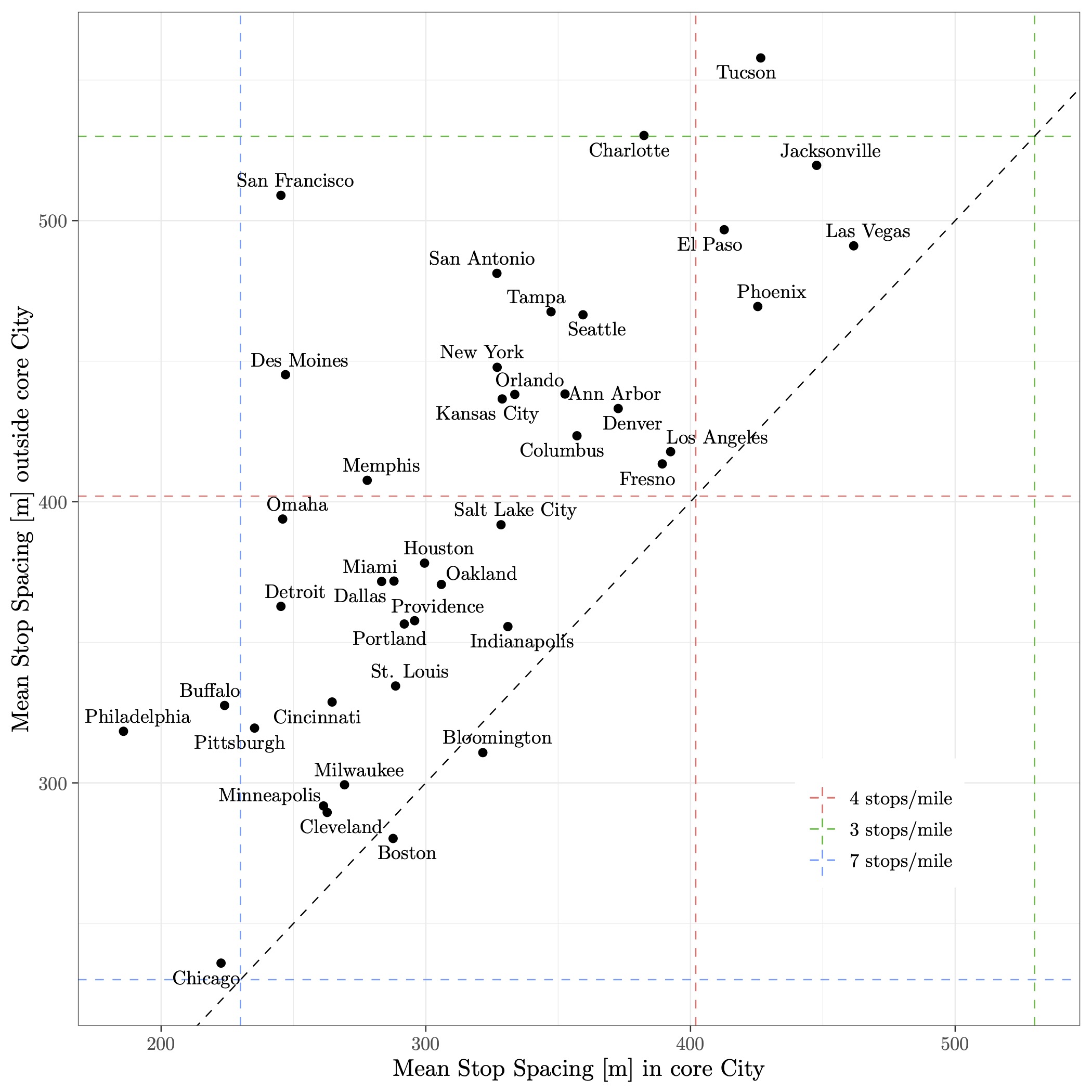
The database can also be combined with geographic data, since we include the locations of both stops in each spacing. As a simple illustration, we use city boundary shapefiles downloaded from Centers for Disease Control and Prevention (2020) to calculate the mean spacing inside and outside each agency’s “core” city, which we define to be the most populated city that the agency serves. If both stops involved in a traversal fall within the core city, we classify the traversal as being inside the core. The last two columns of Table 2 list the resulting means, and Figure 3 visualizes them. Note several facts. First, spacings are generally larger than 7 per mile, and in some cities within the band of 3 to 4 stops per mile claimed to be typical of European cities. Second, stop spacings are larger outside than inside core cities. Third, cities mostly established before the automobile era (e.g., Cleveland) have relatively smaller spacings.

Figure 3
Figure 3.Average Stop Spacing inside and outside core city

This exercise also demonstrates why it is critical for comparisons to be clear about sourcing. For instance, Chicago’s suburban communities are mainly served by PACE Suburban Bus, but our dataset for Chicago comes from the Chicago-focused CTA; hence, the spacing inside and outside the core are similar.

The authors hope the dataset and code provided can serve many purposes. US agencies have tried to consolidate bus stops—e.g., Pittsburgh most recently (Blazina 2020)—and decision-makers might benefit from knowing how their cities’ spacings compare. Similar data could also be collected for cities in other countries. Spacings may also be classified by census tract to answer questions such as: does stop spacing decline with population and/or job density? It may also be worthwhile for researchers to write code targeted more efficiently at studying stop spacings than gtfs2gps is.


  1. Seattle’s GTFS files combine several agencies’ data: ST - Sound Transit; KCM - King County Metro; CT - Community Transit; KT - Kitsap Transit; PT - Pierce Transit; AT - Access Transportation; DCB - Downtown Circulator Bus

Submitted: July 09, 2021 AEST

Accepted: August 12, 2021 AEST

References

Blazina, Ed. 2020. “Port Authority’s Initial Bus Stop Eliminations Showing on-Time Improvements.” Pittsburgh Post-Gazette, February 23, 2020. https:/​/​www.post-gazette.com/​news/​transportation/​2020/​02/​23/​Port-Authority-bus-stops-on-time-performance-improvements-efficiency-transit/​stories/​202002230032.
Centers for Disease Control and Prevention. 2020. “500 Cities: City Boundaries.” https:/​/​chronicdata.cdc.gov/​500-Cities-Places/​500-Cities-City-Boundaries/​n44h-hy2j/​.
Daganzo, Carlos F, and Yanfeng Ouyang. 2019. Public Transportation Systems. WORLD SCIENTIFIC. https:/​/​doi.org/​10.1142/​10553.
Google Scholar
El-Geneidy, Ahmed M., James G. Strathman, Thomas J. Kimpel, and David T. Crout. 2006. “Effects of Bus Stop Consolidation on Passenger Activity and Transit Operations.” Transportation Research Record, no. 1971, 32–41. https:/​/​doi.org/​10.3141/​1971-06.
Google Scholar
Furth, Peter G, and Adam B Rahbee. 2000. “Dynamic Programming and Geographic Modeling.” Transportation Research Record: Journal of the Transportation 00–0870 (00): 15–22.
Google Scholar
Pandey, Ayush, and Lewis Lehe. 2021a. “Replication Data for: Distributions of Bus Stop Spacings in the United States.” Harvard Dataverse. https:/​/​doi.org/​10.7910/​DVN/​AKDQJQ.
———. 2021b. Stop Spacing Database Code. GitHub.
Google Scholar
Pereira, Rafael H. M., Pedro R. Andrade, and Joao Bazzo. 2020. Gtfs2gps: Converting Transport Data from GTFS Format to GPS-Like Records. R Package Version 1.0-5. Vienna: R Found. Stat. Comput. https:/​/​CRAN.R-project.org/​package=gtfs2gps.
Google Scholar
Reilly, Jack M. 1997. “Transit Service Design and Operation Practices in Western European Countries.” Transportation Research Record: Journal of the Transportation Research Board 1604 (1): 3–8. https:/​/​doi.org/​10.3141/​1604-01.
Google Scholar
Wong, James. 2013. “Leveraging the General Transit Feed Specification for Efficient Transit Analysis.” Transportation Research Record, no. 2338 (January), 11–19. https:/​/​doi.org/​10.3141/​2338-02.
Google Scholar

This website uses cookies

We use cookies to enhance your experience and support COUNTER Metrics for transparent reporting of readership statistics. Cookie data is not sold to third parties or used for marketing purposes.

Powered by Scholastica, the modern academic journal management system