COVID-19, Travel Time Reliability, and the Emergence of a Double-Humped Peak Period

1. Questions

Recently, some studies revealed the relationship between travel time variability (TTV) and average travel time based on macroscopic fundamental diagrams (MFD) in urban traffic networks (Yildirimoglu, Limniati, and Geroliminis 2015; Gayah, Dixit, and Guler 2014). The hysteresis loop in the travel time variability diagram (TTVD) shows that there is a relationship between the travel time variance and the departure time. That is, the trips that depart later in the peak period during congestion offset show a higher travel time variance than trips which depart during congestion onset, with the same mean travel time. This means that the status of the traffic network at different departure times will affect Travel Time Reliability (TTR) under the assumption that people’s travel behaviour is unchanging. More interestingly, there is a strong correlation between the hysteresis loop in the TTVD and the hysteresis loop in the MFD, and when the network traffic and density exceed the critical points, TTV will increase sharply (Hemdan, Wahaballa, and Kurauchi 2019).

However, one of the reasons why the hysteresis loop appears in the MFD is because under the same average network density, the temporal and spatial distribution of network congestion differs (Geroliminis and Sun 2011). Therefore, the temporal and spatial distribution of congestion may also explain the appearance of the hysteresis loop in the TTVD. Some studies explored the relationship between the temporal and spatial distribution of congestion and the hysteresis loop in the MFD, as well as the relationship between TTR and the MFD (Saberi and Mahmassani 2012; Mahmassani, Hou, and Saberi 2013), but were limited to small networks with two links, and did not directly give the relationship between the temporal and spatial distribution of congestion and TTR.

In this paper, we investigate the relationship between the temporal and spatial distribution of congestion and TTR in large networks, and ask:

• Is the heterogeneity of spatial-temporal distribution of congestion related to travel time variance, and will it affect TTR?

• Whether and how COVID-19 affected the TTR of the transport network?

2. Methods

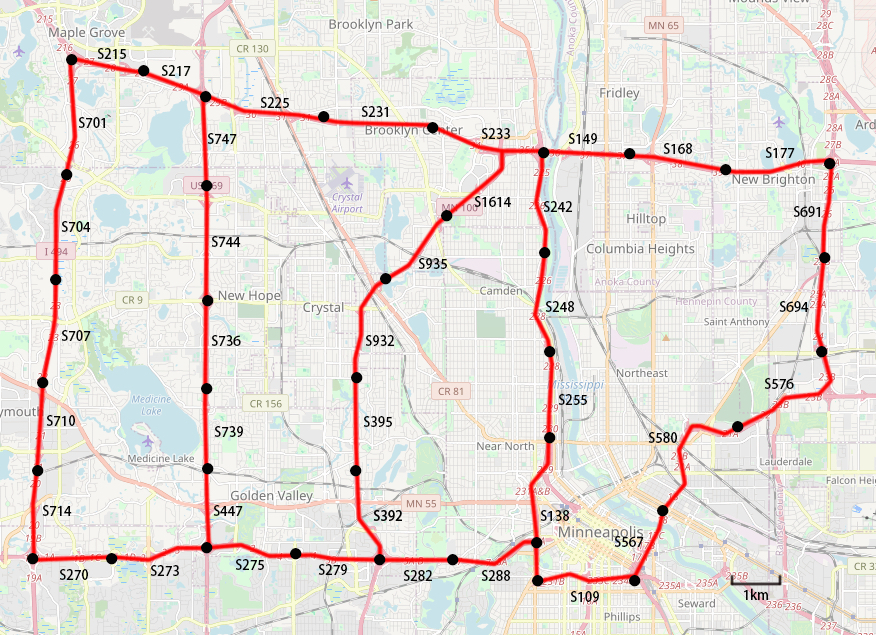
We chose the Minneapolis-St.Paul freeway network in Minnesota, which displays a grid-like network topology and includes links in series and parallel, as shown in Figure 1. The selected sub-network has 39 traffic segments (each around 2 km) and corresponding detectors on the mainline freeways, which are located on major highways in the northwestern suburbs. The selected morning peak period runs from 6:00 am to 9:00 am and the 5-minute loop detector data for all working days from January 1 to May 31 in the three years of 2019, 2020 and 2021 come from Mn/DOT Traffic Data.

Figure 1.The selected sub-network

Following Yildirimoglu and Geroliminis (2013), Yildirimoglu, Limniati, and Geroliminis (2015), the instantaneous travel times of the segments in the network are calculated by a constant speed interpolation method, which means that the segments’ travel times are calculated by the mean of the speed at two consecutive detectors at the current departure time period. The travel time mean ($\mu(t)$) and variance ($\sigma^2(t)$) of the whole network are given in Equation 1 and Equation 2, which indicates the TTR of the network.

$$\mu_{j}(t)=\frac{1}{I}\sum_{i=1}^{I}\tau_{ij}(t) \tag{1}$$

$$\sigma^2(t)=\frac{1}{I-1}\sum_{j=1}^{J}\sum_{i=1}^{I}(\tau_{ij}(t)-\mu_{j}(t))^2 \tag{2}$$

where $t$ is five-minute departure time interval, $I$ is the number of days, $J$ is the number of segments in the network and $\tau_{ij}(t)$ is the travel time within the network segment $j$ at departure time $t$ on the day $i$.

The occupancy indicates the percentage of time a detector’s field is occupied by a vehicle (Minnesota Department of Transportation 2021), and the greater the occupancy, the greater the congestion. In the rest of this paper, to avoid confusion, occupancy and congestion have the same meaning. The spatial heterogeneity of network occupancy in the departure time period is indicated in Equation 3 and Equation 4.

$$\nu_{i}(t)=\frac{1}{J}\sum_{j=1}^{J}o_{ij}(t) \tag{3}$$

$$\omega^2(t)=\frac{1}{I}\cdot\frac{1}{J} \sum_{i=1}^{I}\sum_{j=1}^{J}(o_{ij}(t)-\nu_{i}(t))^2 \tag{4}$$

where $o_{ij}(t)$ is the occupancy within the network segment $j$ at five-minute departure time interval $t$ on the day $i$, $\nu_{i}(t)$ is the mean occupancy of all segments in the network at departure time $t$ on the day $i$ and $\omega^2(t)$ is the indicator of the spatial heterogeneity of network occupancy.

Traffic flow can reveal the transport capacity of the network, and it can also reflect the travel demand of the area (Parthasarathi et al. 2011). The average traffic flow in the network is indicated in Equation 5.

$$q(t)=\frac{1}{J}\cdot\frac{1}{I}\sum_{i=1}^{I}\sum_{j=1}^{J}f_{ij}(t) \tag{5}$$

where $f_{ij}(t)$ is the traffic flow (all lanes together) measured by detector within the segment $j$ at five-minute departure time interval $t$ on the day $i$, $q(t)$ is the average traffic flow of the network at departure time $t$.

3. Findings

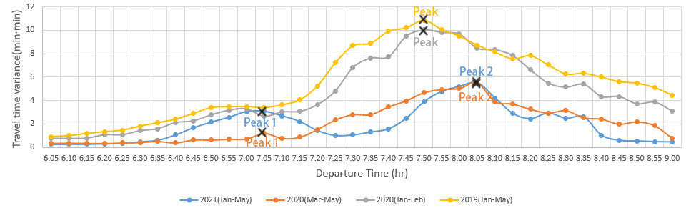
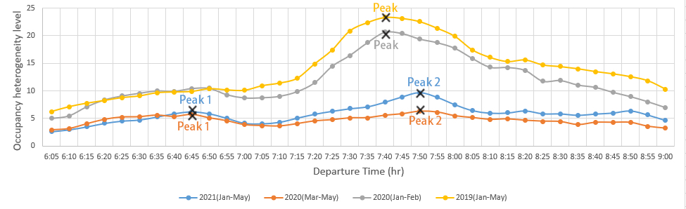
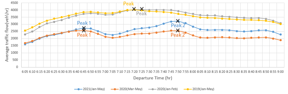
From Equation 2, Equation 4 and Equation 5, we can obtain travel time variance, network occupancy heterogeneity level, and average traffic flow vs. departure time for 2019, 2020, and 2021. Considering that the lockdown in 2020 occurred in March, the 2020 data is divided into two parts: January-February and March-May. Results are shown in figures 2, 3 and 4.

Figure 2.Travel time variance ($\sigma^2(t)$) during morning peak period in 2019, 2020 and 2021

Figure 3.Occupancy heterogeneity ($\omega^2(t)$) level during morning peak period in 2019, 2020 and 2021

Figure 4.Average traffic flow ($q(t)$) during morning peak period in 2019, 2020 and 2021

We observe that before the pandemic, the changes in network travel time variance, occupancy heterogeneity level and average traffic flow in Jan to May 2019 and Jan to Feb 2020 showed a dominant single-humped pattern during the morning peak period. However, after the pandemic, they showed a double-humped pattern in Mar to May 2020 and Jan to May 2021, and compared with 2020, this pattern is even more pronounced in 2021. We believe this is because the impact of the pandemic on travel demand and mode was not yet fully formed in 2020.

In addition, the dynamic changes of occupancy heterogeneity level and average traffic flow are almost at the same time of day, but they are earlier than travel time variance, that is, there is a hysteresis between them. Some key information of these three network characteristics are summarized in Table 1, with the value in brackets representing the time when the peak occurred.

From Table 1, we see the peak occurrence time of occupancy heterogeneity level and average traffic flow is 10-20 min earlier than the travel time variance. The reason is that the overall travel demand in the region is changing from the onset of the morning peak period, and this change leads to a change in the level of heterogeneity of occupancy.

The increase in the level of heterogeneity of occupancy means that severely congested segments begin to appear in the network. These segments will increase the uncertainty of travel conditions in the subsequent time periods, thereby reducing the travel time reliability and increasing travel time variance. This answers the first question that the heterogeneity of the temporal and spatial distribution of traffic occupancy is related to the variance of travel time and will affect TTR.

Regarding the second question, TTR is indeed affected by COVID-19, because COVID-19 affected people’s travel demands and travel patterns, which is reflected in the change from single to double-humped, and this impact became more significant from 2020 to 2021. From Table 1, we find that before and after COVID-19, the average network traffic flow during the morning peak period dropped from 3,531 veh/hr in 2019 to 2,544 veh/hr in 2021, which also led to a decrease in the level of network occupancy heterogeneity. As a result, the average travel time variance during the morning peak period decreased from 5.43 $min^2$ in 2019 to 1.94 $min^2$ in 2021. There is no doubt that the pandemic has led to an increase in the TTR.

We believe the reason for the emergence of the double-humped pattern is the changing composition of the commuting workforce. According to data (Minnesota Compass 2021), the total number of all jobs in Minnesota has been reduced by 6.8% in 2020 after the COVID-19 outbreak. Among them, construction and natural resources and mining industry decreased by 2.48% and 0.18% respectively, which are the industries least affected by the pandemic. The commonality of these two industries is that they go to work early and cannot work remotely. Therefore, office workers who tended to travel to work later in the peak period and dominated the number of travelers in the morning commute pre-COVID began working from home in large numbers, while many non-office workers, who would tend to travel earlier have not stopped commuting and so now comprise a larger share of commuting travelers, has lead to the emergence of the second peak on these curves. Different types of workers always had different start times, but this was masked by the dominance of the 8:00-8:30 am start time, and is now revealed with the shifting composition of the commuting workforce.

Acknowledgments

The author thanks the Minnesota Department of Transportation for providing relevant data sets.