
1. QUESTIONS
Around Seoul, suburbanization has accelerated through new town development, and commuting into the city has increased, making congestion worse. GTX (Great Train eXpress, top speed 180 km/h; Ministry of Land, Infrastructure and Transport 2024) is an attempt to address this through expanding public transport. A faster line changes travel in and out of the suburbs, including commuting. Excess commuting measures how inefficient that commuting is. Therefore, whether a faster line shortens commuting or lets commuters reach farther jobs can be measured by excess commuting: the distance or time by which a district’s commuting goes beyond what the locations of homes and jobs require (Hamilton 1982; Ma and Banister 2006a; White 1988).
GTX-A, the first GTX line, opened its northern section on 28 December 2024. Paju district, at the northern end of the line, has a new town, Unjeong, which is still growing: the town’s population grew from 268,000 in 2023 to 303,000 in 2025 (Ministry of the Interior and Safety 2026; Supplemental Information). The GTX-A station opened inside the town, and the line cut the trip to Seoul Station from 46 minutes by rail and 66 by express bus to 22 minutes (Ministry of Land, Infrastructure and Transport 2024). Paju therefore offers a unique opportunity to observe the two changes that move excess commuting at the same time: the opening changed travel times to Seoul on one day, and the new town keeps changing the locations of homes and jobs as it fills with new residents. Many studies have followed how excess commuting changes over time (Chen et al. 2023; Ma and Banister 2006b, 2007; Murphy 2016; Yang 2008; Zhou and Murphy 2019). However, no study has measured what the opening of a fast rail line does to excess commuting. In this paper, we ask whether excess commuting at Paju changed, in distance or in time, how it evolved month by month, and where the added commuting goes. We measure the excess in two steps: with the numbers of resident workers and jobs in each zone held at their pre-opening levels, so that only a change in where commuters work can move the excess, and then with those numbers following each month, so that the minimum commute follows new residents and their workplaces as well.
2. METHODS
The data are the Seoul capital region’s de facto population mobility data (Seoul Metropolitan Government and KT 2025): daily origin–destination flows inferred from mobile network signals, each with an inferred trip purpose. In mobile phone data generally, purpose is inferred more accurately for commuting than for other trips, because home and work are regularly located day by day (Abdi et al. 2026). We use work trips by domestic residents for Tuesday to Thursday during one mid-month week per month, January 2023 to December 2025.
Excess commuting is measured against the transportation problem (White 1988). Let Oi be the resident workers of zone i (Seoul’s 426 dong, its neighbourhood zones, and the 52 districts outside Seoul; Supplemental Information), Dj the jobs taken in zone j, mijt the observed commuters from zone i to zone j in month t, and cij the pair’s mean reported distance (or time) in 2023, before any GTX section opened. The least-cost assignment x minimises
\[ \Sigma_i \Sigma_j x_{i j} c_{i j} \quad \text { subject to } \quad \Sigma_j x_{i j}=O_i, \quad \Sigma_i x_{i j}=D_j, \quad x_{i j} \geqslant 0 . \]
We solve it in two steps. In the first step Oi and Dj are their 2024 means and the assignment is solved once, so that only a change in where commuters work can move the excess. In the second step Oi and Dj are each month’s own, so that the minimum commute follows new residents and their workplaces as well. Excess at origin i in month t is
\[ E_{i t}=\Sigma_j m_{i j t} c_{i j} / \Sigma_j m_{i j t}-\Sigma_j x_{i j} c_{i j} / O_i, \]
that month’s actual mean commute less the minimum commute. An origin’s minimum commute is its share of this region-wide assignment. We confirmed that this assignment has a unique solution in every month (Supplemental Information). Excess time is measured at 2023 travel times, which reflect only the mix of destinations, and at actual travel times, those reported for each month, which also reflect faster travel (the assignment solved again each month).
Outside Seoul the capital region has 52 districts, six with GTX-A stations; we report Paju. The comparison group is the remaining 46 less two whose pre-opening excess was not positive, leaving 44 districts. Because the level of excess depends on zone size (Small and Song 1992), each estimate is Paju’s own change in excess, in percent of its pre-opening level, less the change in the comparison districts’ median, twelve months after the opening against twelve months before. Its 95% interval comes from a moving-block bootstrap of the monthly gaps between Paju’s excess and the comparison median, both in percent of their pre-opening levels, and p from the estimate’s rank in absolute value among all 45 districts (Supplemental Information). The interval measures how precisely the twelve-month difference is estimated from the month-to-month variation of Paju’s gap; p asks whether Paju’s estimate is significantly different from those of the districts without a station.
3. FINDINGS
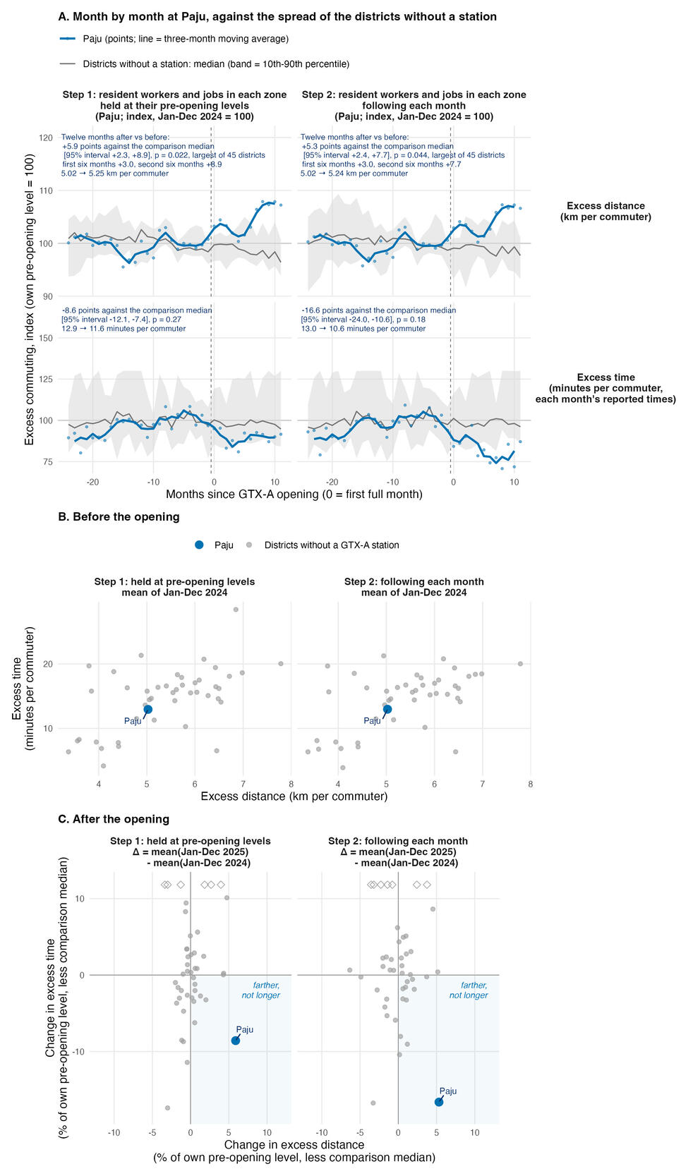
Figure 1A shows that Paju’s excess distance rose in both steps. With the numbers of resident workers and jobs in each zone held fixed, it rose 5.9 points of its pre-opening level against the comparison median (95% interval 2.3 to 8.9), and this rise was the largest among the 45 districts (p = 0.022). With those numbers following each month, it rose 5.3 points (95% interval 2.4 to 7.7), and this rise was also the largest, although one comparison district’s fall was larger in absolute value (p = 0.044): the minimum commute rose only 0.017 km, so the two steps give nearly the same distance. Paju’s gap from the comparison median was already widening before the opening, by 0.37 points a month over 2024 and 0.10 over 2023 and 2024 in the first step and by 0.22 and 0.06 in the second; projecting each step’s own drift through the post-opening year leaves 1.5 and 4.9 of the first step’s 5.9 points (p = 0.58 and 0.067) and 2.6 and 5.0 of the second step’s 5.3 (p = 0.51 and 0.13), so the rise is a post-opening association of 1.5 to 5.9 points depending on the trend assumed (Supplemental Information). Excess time at actual travel times fell in both steps, 8.6 points in the first and 16.6 in the second, neither significantly different from the comparison districts (p = 0.27 and 0.18). It fell more in the second step because resident workers grew faster than jobs, so the minimum commute rose about 1 minute. At 2023 travel times, which hold speeds fixed, excess time rose in the first step (+6.2 points, p = 0.022) and fell in the second (−3.2 points, not significantly different from the comparison districts, p = 0.40), again because the minimum commute rose (Supplemental Information). Figure 1B shows that before the opening Paju’s excess was below the median of the 45 districts, in distance (5.0 km against 5.5) and in time at actual travel times (12.9 minutes in the first step against 15.6). Figure 1C shows that Paju alone combines a large rise in excess distance with a fall in excess time, in both steps.
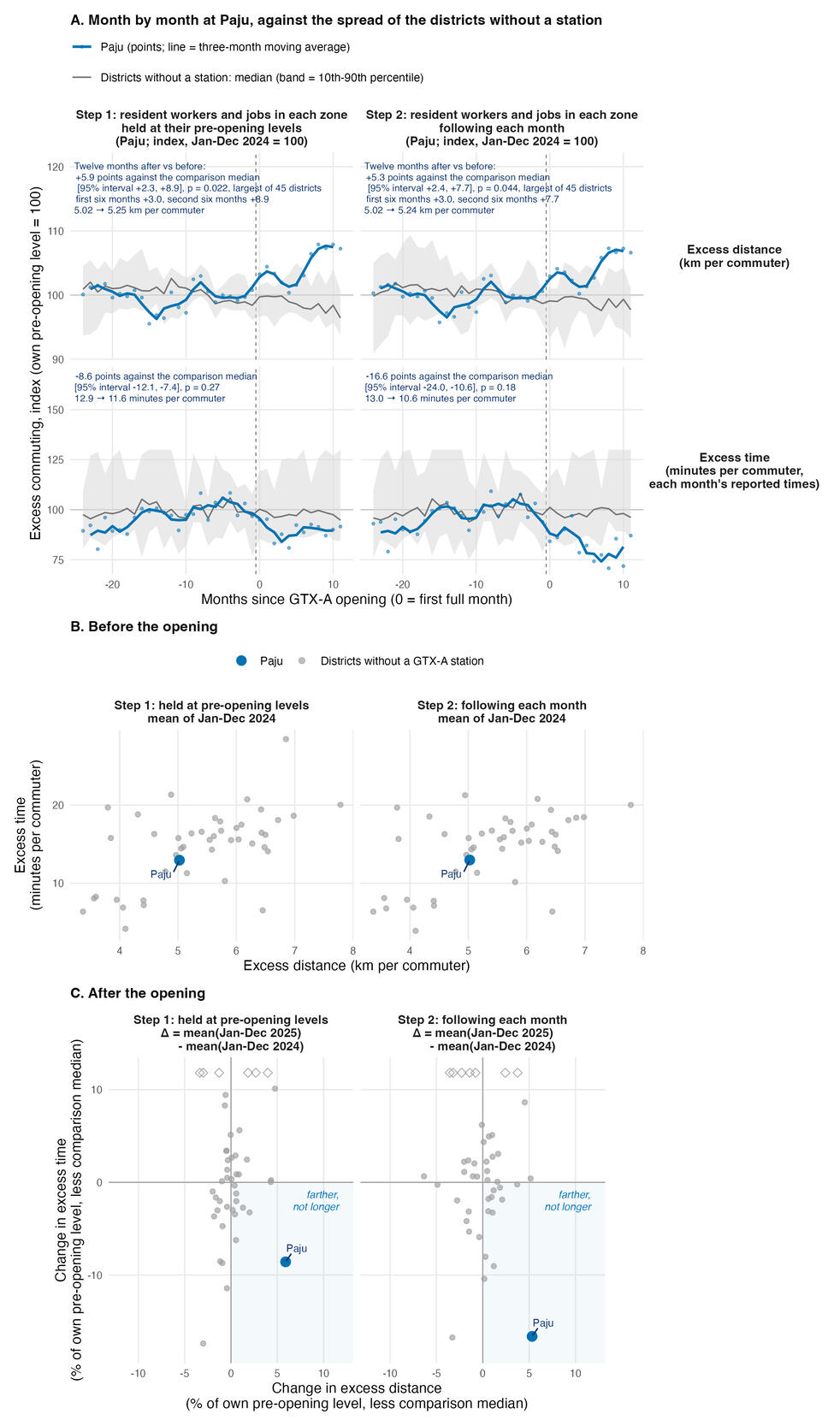
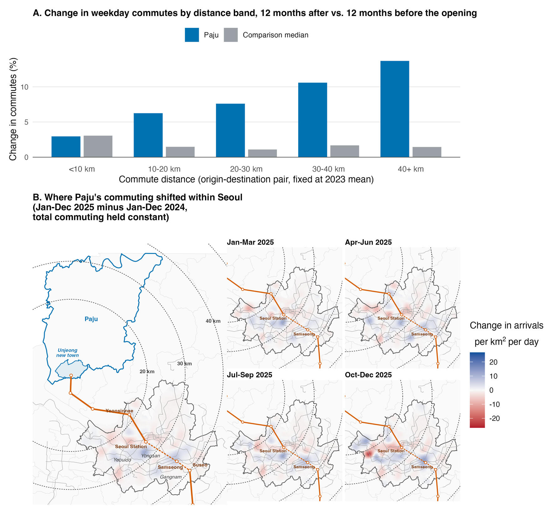
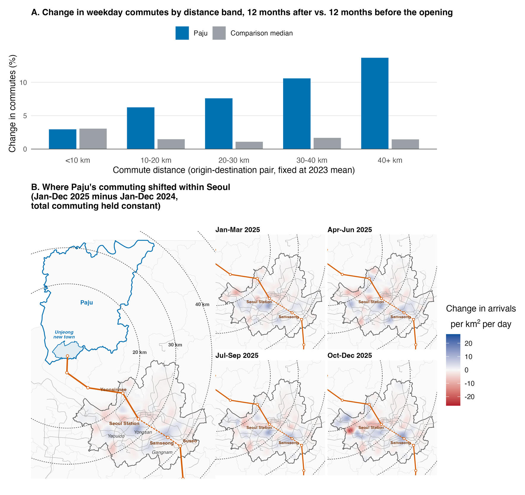
Figure 2 counts observed commutes, which are the same in both steps. Figure 2A shows that the added commuting goes to longer distances: commutes below 10 km grew only 3.0%, while those beyond 40 km grew 13.7%. Commuting to Seoul grew 9.5% against a comparison median of 1.1%. The growth was as much within 3 km of the open stations, Seoul Station and Yeonsinnae (10.1%), as beyond 3 km (9.4%). The strongest increases on the map are at the Yongsan business district beside Seoul Station and at Yeouido, the financial district (Figure 2B). Growth was fastest toward the Gangnam business district, which the line does not directly reach yet: commuting within 3 km of Samseong or Suseo station grew 19.1% against a comparison median of 1.7%. The actual travel time from Paju to that area fell 7.1 minutes against 0.3 from the comparison districts pooled, as a first leg by GTX-A would produce; the data do not record route or mode (Supplemental Information).
After the opening, the mean commute distance of Paju’s commuters grew 2.9 points of its pre-opening level against the comparison median, and this rise was the largest among the 45 districts (p = 0.022). The change in their mean commute time was not significant (+1.2 minutes; +2.2 points against the comparison median, 95% interval −1.0 to +5.2, p = 0.24; Supplemental Information), so the evidence is stronger for a change in where commuters work than for a change in how long their trips take. These results are consistent with previous studies on travel time, which found that at the aggregate level trip distances grow with travel speeds while travel times remain stable (Levinson and Kumar 1994; Mokhtarian and Chen 2004). In addition, excess commuting shows that, in distance, the added commuting goes beyond what the locations of Paju’s homes and jobs require. The data are monthly flows, not people, so existing residents changing jobs cannot be distinguished from new residents taking farther ones; but Unjeong filled as fast in 2024 as in 2025 and Paju’s commuter count did not grow significantly faster than the comparison districts (Supplemental Information).
ACKNOWLEDGMENTS
The authors designed the study, carried out the analysis, and take responsibility for the content. Anthropic Claude and OpenAI Codex assisted with drafting, code, and consistency checks; the authors independently verified all analytical decisions, code, and interpretations.
DATA AND CODE
The mobility data are open data of the Seoul Metropolitan Government (Seoul Open Data Plaza, dataset OA-22300). A single R script that downloads the sampled days and reproduces every result computed from the mobility data in the text and in the Supplemental Information, and Figure 1 and Figure S2, is available at https://github.com/knugislee1/gtx-excess-commuting (Supplemental Information, S5).
CONFLICT OF INTEREST
The authors declare no conflict of interest. No external funding supported this work.