Speed Limit Changes and Driver Behaviour: A Spatial Lag Model

Research Question and Hypothesis

The lack of compliance to speed limits is pervasive. Typically, 40 % to 50 % of motorists drive above the speed limit (OECD/ECMT 2006). Speed is an essential factor in road safety because it directly affects the frequency and severity of crashes (Aarts and Van Schagen 2006; FHWA 2017). Driver behaviour is influenced by many external factors such as road design, road environment, traffic control devices, the presence of other vehicles, and weather conditions (Gargoum, El-Basyouny, and Kim 2016; Goldenbeld and van Schagen 2007; Wilmot and Khanal 1999). Transport authorities try to change the drivers’ behaviour through education, speeding controls, changes to the road design or road environment, and through technology such as driver assistance systems in vehicles (Wallén Warner and Åberg 2008). However, the effects of these measures are often limited in time and space (Comte, Varhelyi, and Santos 1997). This paper examines speed choice by drivers in response to a change in the speed limit without any known modification to the road design and the immediate environment. This paper tests whether driving speed is spatially correlated and compares two statistical models, a regular linear model, and a spatial lag model.

Methods and data

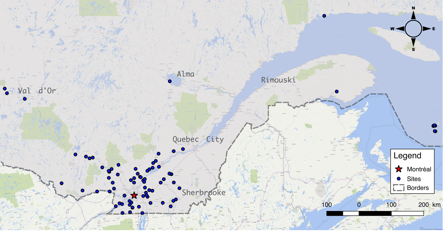
In total, 76 road segments (sites) with a decrease (n=12) or an increase (n=64) of their speed limit between 2006 and 2017 were analysed, over a period of six years before and after the speed limit changes. Those sites are located across the province (see Figure 1). The targeted road segments are provincial highways (national, regional, and collector roads), excluding local roads and freeways.

Figure 1:Map illustrating the location of study sites where a speed limit change occurred (n=76)

First, the individual vehicle speed data were collected at the study sites by the Quebec Ministry of Transportation (MTQ) and the research team. For each site, speeds were recorded at different periods, usually for three to five consecutive days at a time, before and after the change (the records done by the research team were only three hours, following the MTQ guidelines). There are between 2 and 17 records at each site. Only free-flow speeds are used in this analysis.

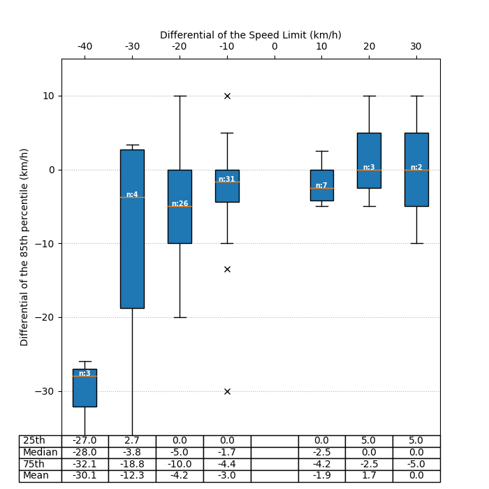
Figure 2 illustrates the differential of the 85^th percentile of the average speeds (after minus before) per site according to the change in speed limits. This figure shows the non-linear pattern of the changes in speed behaviour by the drivers according to the speed limit change: drivers do not all comply with the speed limit, nor do they adjust their speed according to the magnitude of the speed limit change.

Figure 2:Boxplots of the differentials of the 85^th percentile of the average speeds according to the speed limits change (n indicating the number of sites)

Secondly, for each road segment and period during which speed was recorded, data about the road design and environment were extracted from public spatial databases. These explanatory (independent) variables are described in Table 1. To select an appropriate model using these variables, we applied the stepwise model selection procedure, which automatically selects the best subset of variables from a pool of candidates using the AIC (Akaike Information Criterion).

The speed ratio, defined as the average speed for each speed record divided by the speed limit, is the dependent variable. It is used to compare the average operating speeds between sites that do not have the same speed limit (Morency et al. 2017). Since the speed behaviour of drivers is influenced by other drivers and the road environment, the social interactions and culture, there may be some spatial correlations between the observed speeds. Unlike linear models, a spatial model considers the neighborhood effect of observations. The model (with the spatial lag) can be represented as

$$Y_{i} = \rho\sum_{j = 1}^{n}{w_{\text{ij}}Y_{j}} + X_{i}\beta + \epsilon_{i},\epsilon_{i}\sim\text{N}\left( 0,\sigma^{2} \right),\hspace{20mm}(1)$$

where $Y_{i}$ is the speed ratio at site $i$, $X_{i}$ is the vector of variables for the site i, $\beta$ the vector of coefficients, $w_{\text{ij}}$ the spatial weight for sites i and j, $\rho$ a spatial autoregression scalar parameter, the errors $\epsilon_{i}$ are supposed to be normally distributed with standard deviation $\sigma$ and n is the number of sites. $\rho = 0$ depicts a lack of spatial correlation, while $\rho \neq 0$ implies a positive or negative spatial autocorrelation between neighboring sites. For a proper treatment of spatial linear model and their variations, see Diggle (2003) and Bivand, Pebesma, and Gómez-Rubio (2013), among others.

To examine the spatial autocorrelation in the data, i.e., test whether a variable at one site depends on neighboring observations, the spatial autocorrelation for a variable $y_{i}$ can be measured through Moran’s I:

$$I = \frac{n\sum_{i = 1}^{n}{\sum_{j = 1}^{n}{w_{\text{ij}}\left( y_{i} - \overline{y} \right)\left( y_{j} - \overline{y} \right)}}}{\sum_{j = 1}^{n}{w_{\text{ij}}\left( y_{i} - \overline{y} \right)^{2}}}\hspace{20mm}(2)$$

The hypothesis that Moran’s I is 0 can be tested (Bivand (2019)): a positive (resp. negative) spatial autocorrelation indicates that similar (resp. dissimilar) values appear close (resp. far) to each other in space. There are different methods to compute the spatial weights $w_{\text{ij}}$ (Bivand, Pebesma, and Gómez-Rubio (2013)): here, two sites are neighbour within a reasonable maximum distance of influence (a threshold of 50 km was chosen based on the distribution of site distance by some trial and error). Three sites have no neighbour, and other sites have 4.9 neighbours on average. If there is spatial correlation for the speed ratio and for the spatial correlation of the residuals of a regular linear model, a spatial model can be fitted to the data.

Findings

Moran’s I for the speed ratio is -0.053 ($p < 0.001$). A spatial and regular model were therefore fitted to the selected explanatory variables, only for the 49 sites with reduced speed limits. Moran’s I for the residuals of the regular model is -8.860 ($p < 0.001$). The estimated parameters of the proposed models are presented in Table 2. The spatial autoregression parameter, $\rho = - 0.114$ ($p < 0.001$), which implies a negative spatial autocorrelation between neighboring sites. Furthermore, comparing the spatial and regular models in terms of AIC shows the spatial regression provides a better fit to the data. The models are very similar, with the same coefficient signs and the same significant variables (except for the year 2011). Most of the variable associations with the speed ratio are expected. There is an increase in the speed ratio after a speed limit decrease, which means that driving speed increases relative to the speed limit and is consistent with Figure 2. This increase is larger in urban areas based on the area and distance to the nearest city center. Road features like side curbs, lateral and median strips are associated with lower speed ratios and may be used as traffic calming measures. There is no clear temporal trend.

Our results demonstrate that speeds are spatially correlated. It also confirms that drivers only partly adjust their speeds after a speed limit change. More research is needed to understand how to increase compliance and how social and cultural factors may play a role in driving speed.

Acknowledgment

We acknowledge the financial support provided by the Quebec Ministry of Transportation (MTQ: Project R794.1) and the work of Gaëtan Dussault on the spatial database.

References

Aarts, Letty, and Ingrid Van Schagen. 2006. “Driving Speed and the Risk of Road Crashes: A Review.” Accident Analysis & Prevention 38 (2): 215–24. https:/​/​doi.org/​10.1016/​j.aap.2005.07.004.
Google Scholar
Bivand, R.S. 2019. “Spdep: Spatial Dependence: Weighting Schemes, Statistics and Models.” https:/​/​cran.r-project.org/​web/​packages/​spdep/​spdep.pdf.
Bivand, R.S., E. Pebesma, and V. Gómez-Rubio. 2013. Applied Spatial Data Analysis with R. Springer Science & Business Media.
Comte, S., A. Varhelyi, and J. Santos. 1997. “The Effects of ATT and Non-ATT Systems and Treatments on Driver Speed Behaviour.” Espoo, Finland.
Diggle, P.J. 2003. Statistical Analysis of Spatial Point Patterns. London: Edward Arnold.
FHWA. 2017. “Road Safety Fundamentals: Concepts, Strategies, and Practices That Reduce Fatalities and Injuries on the Road (FHWA-SA-18-003.” Washington, DC.
Gargoum, Suliman A., Karim El-Basyouny, and Amy Kim. 2016. “Towards Setting Credible Speed Limits: Identifying Factors That Affect Driver Compliance on Urban Roads.” Accident Analysis & Prevention 95 (October):138–48. https:/​/​doi.org/​10.1016/​j.aap.2016.07.001.
Goldenbeld, Charles, and Ingrid van Schagen. 2007. “The Credibility of Speed Limits on 80km/h Rural Roads: The Effects of Road and Person(Ality) Characteristics.” Accident Analysis & Prevention 39 (6): 1121–30. https:/​/​doi.org/​10.1016/​j.aap.2007.02.012.
Morency, C., M. Trépanier, N. Saunier, M.-A. Tessier, J. Faucher, J.-S. Bourdeau, and A. Giraud. 2017. “Projet de recherche sur le développement d’un outil de suivi et d’analyse des conditions de circulation sur le réseau routier du MTMDET de la région de Montréal.” http:/​/​www.bv.transports.gouv.qc.ca/​mono/​1200488.pdf.
OECD/ECMT. 2006. Speed Management. Paris: OECD Publishing.
Wallén Warner, Henriette, and Lars Åberg. 2008. “Drivers’ Beliefs about Exceeding the Speed Limits.” Transportation Research Part F: Traffic Psychology and Behaviour 11 (5): 376–89. https:/​/​doi.org/​10.1016/​j.trf.2008.03.002.
Wilmot, Chester G., and Mandar Khanal. 1999. “Effect of Speed Limits on Speed and Safety: A Review.” Transport Reviews 19 (4): 315–29. https:/​/​doi.org/​10.1080/​014416499295420.
This website uses cookies
We use cookies to enhance your experience and support COUNTER Metrics for transparent reporting of readership statistics. Cookie data is not sold to third parties or used for marketing purposes.
Powered by Scholastica, the modern academic journal management system