This website uses cookies

We use cookies to enhance your experience and support COUNTER Metrics for transparent reporting of readership statistics. Cookie data is not sold to third parties or used for marketing purposes.

Skip to main content
null
Findings
  • Menu
  • Articles
    • Energy Findings
    • Resilience Findings
    • Safety Findings
    • Transport Findings
    • Urban Findings
    • All
  • For Authors
  • Editorial Board
  • About
  • Blog
  • search
  • X (formerly Twitter) (opens in a new tab)
  • LinkedIn (opens in a new tab)
  • RSS feed (opens a modal with a link to feed)

RSS Feed

Enter the URL below into your favorite RSS reader.

https://findingspress.org/feed
ISSN 2652-8800
Transport Findings
November 03, 2026 AEST

Whose Time Do Traffic Signals Save? Pedestrian–Vehicle Delay Tradeoffs Across Sydney Intersections

David M. Levinson, Ph.D.,
pedestrian delayvehicle delaytraffic signalsmodal comparisonsignal timingtime allocation
Copyright Logoccby-sa-4.0 • https://doi.org/10.32866/001c.172237
Findings
Levinson, David M. 2026. “Whose Time Do Traffic Signals Save? Pedestrian–Vehicle Delay Tradeoffs Across Sydney Intersections.” Findings, November 2. https://doi.org/10.32866/001c.172237.
Save article as...▾
Download all (4)
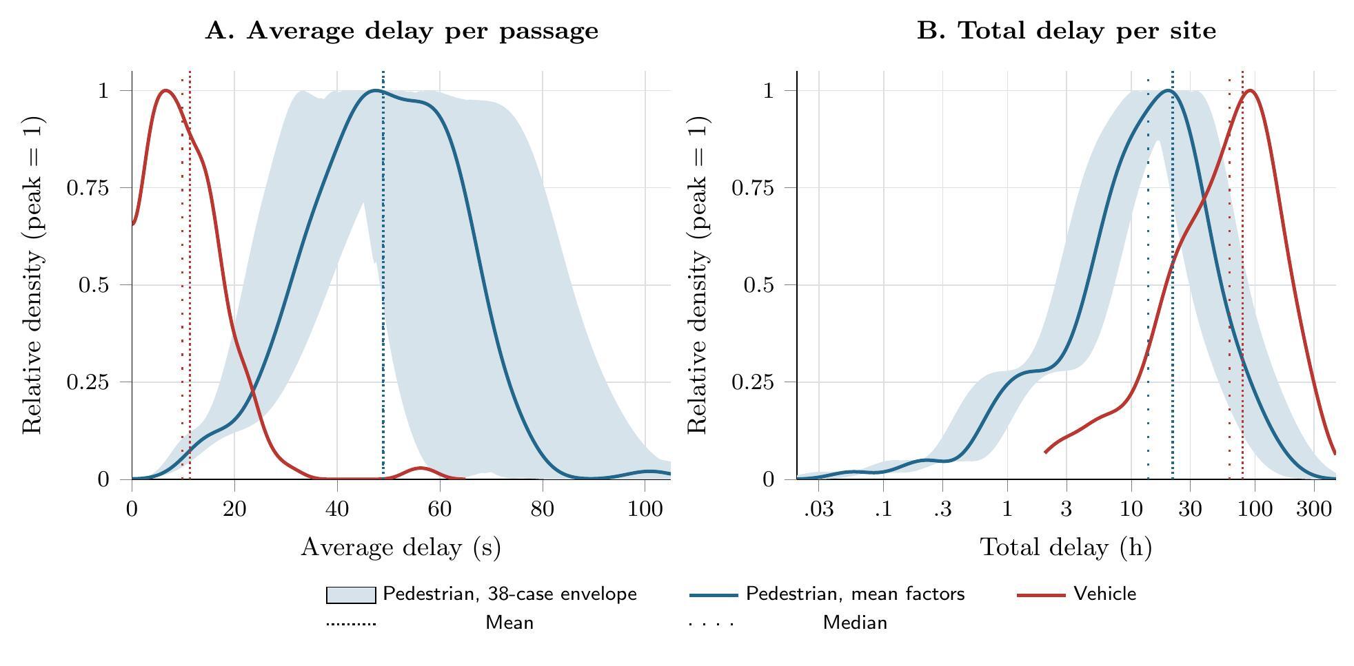
  • Figure 1. Peak-normalized site distributions under full Walk compliance; each curve has maximum height one, so the panels compare shapes rather than density magnitude. Panel A shows mean pedestrian delay in seconds per estimated crossing (blue; mean 48.98, median 48.88) and mean vehicle delay per detected vehicle (red; mean 11.28, median 9.77). Panel B shows pedestrian person-hours (blue; mean 21.62, median 13.66) and vehicle-hours (red; mean 79.04, median 62.43). Dense dotted lines mark unweighted site means and loose dotted lines mark medians. The 39.8-second value in the text is the crossing-weighted network mean pedestrian delay. Each of the 38 pedestrian calibration curves is normalized separately before forming the pale-blue envelope; the aggregate average-delay ratio remains 2.685–4.788 (SI-4). Vehicle estimates do not use pedestrian calibration.
    Download
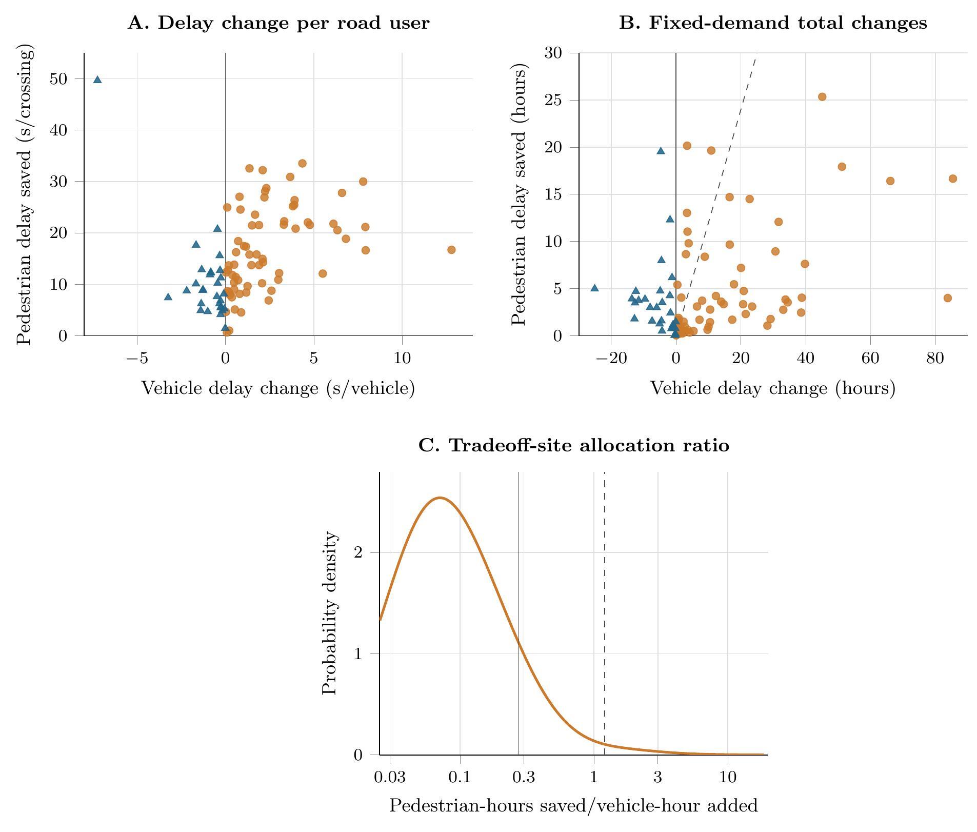
  • Figure 2. Thirty-second-cap fixed-count results using mean factors and full Walk compliance. Panel A reports seconds per estimated crossing and detected vehicle. Orange circles are the 66 vehicle-cost sites; blue triangles are the 29 sites where both modes save time. In Panel B, the dashed line is zero equal-clock-time balance at occupancy 1.2. Panel C shows pedestrian-hours saved per vehicle-hour added; the solid line is the 0.274 median and the dashed line is the equal-weight break-even value at occupancy 1.2.
    Download
  • Code and analysis outputs
    Download
  • Supplemental Information (PDF)
    Download

Error

Sorry, something went wrong. Please try again.

If this problem reoccurs, please contact Scholastica Support

Error message:

undefined

View more stats

Abstract

At 168 Sydney intersections, estimated pedestrian delay averages 39.8 seconds per crossing if everyone waits for Walk, or 29.8 seconds under observed crossing behavior, compared with 10.4 seconds per detected vehicle. We test earlier pedestrian service while holding pedestrian and vehicle volumes at their current levels. With a 30-second first-call wait target, the 95-site experiment saves 440 pedestrian-hours but adds 886 vehicle-hours, assuming full Walk compliance. At 1.2 occupants per vehicle, pedestrian waiting must count more than 2.42 times as much as vehicle-occupant waiting for the weighted time savings to exceed the added delay. In the seven-day experiment at 35 intersections, the weighted time savings exceed the added delay when pedestrian waiting counts more than 2.22 times as much as vehicle-occupant waiting.

1. Questions

Traffic signals divide waiting time between pedestrians and vehicles. The Sydney Coordinated Adaptive Traffic System (SCATS) records pedestrian-button requests, signal states, and vehicle-detector counts (Transport for NSW 2024). These records identify the first accepted button request after flashing-don’t-walk begins, which we call the first actuation. They do not identify pedestrians who arrive later. Earlier studies estimate pedestrian delay from controller events (Karimpour et al. 2022) and optimize signal timing for pedestrians and vehicles together (Roshandeh et al. 2014; Yu et al. 2017; Liang et al. 2020). We ask:

  1. How do average and total pedestrian delay compare with vehicle delay at the same intersections and during the same hours?

  2. How would delay change for each mode if pedestrian service began earlier, aiming to limit the wait after the first button request to 15, 20, 30, or 45 seconds?

2. Methods

We link SCATS pedestrian-button requests, Walk indications, signal phases, vehicle green intervals, and detector counts for Tuesday, 18 September 2018, an arbitrarily selected date. Each site-hour represents one intersection during one clock hour. The comparison of current conditions covers 2,226 site-hours at 168 intersections. Of these intersections, 95 meet the criteria for the 30-second timing experiment. We also repeat the analysis for 14–20 September at 35 intersections with complete inputs for all seven days. Supplemental Information describes the study-day weather and the limits of these samples.

The companion network study uses the timing of the first button request to estimate arrival events \(\widehat N_{sh}^{p,e}\) and their accumulated delay \(\widehat D_{sh}^{p,e}\) at site \(s\) during hour \(h\) (Levinson 2026a). An arrival event can be one pedestrian or a group. Calibration factors from 14 manual-observation and 24 video-observation cases convert arrival events to individual crossings and event-delay to pedestrian delay (Levinson 2026b):

\[\widehat N_{sh}^p=\widehat\alpha_N\widehat N_{sh}^{p,e},\qquad \widehat D_{shq}^p=\widehat\alpha_{Dq}\widehat D_{sh}^{p,e},\qquad \widehat{\bar d}_{shq}^p=\frac{\widehat D_{shq}^p}{\widehat N_{sh}^p},\tag{1}\]

Here \(q\in\{100,\mathrm{beh}\}\) distinguishes two estimates: everyone waits for Walk, or pedestrians cross as observed in the calibration data (Choy and Levinson 2026). Across the 38 cases, the mean multipliers are \(\overline{\widehat{\alpha}}_N=2.203\) for crossings, \(\overline{\widehat{\alpha}}_{D,100}=2.212\) for full-compliance delay, and \(\overline{\widehat{\alpha}}_{D,\mathrm{beh}}=1.655\) for observed-behavior delay. The ranges show how results vary across calibration cases. They are not confidence intervals and do not capture other sources of uncertainty.

For vehicles arriving on approach \(a\), we assign zero signal delay during green and otherwise assign the time until the next green. This assigned delay is \(r_{ash}^v(t)\). We average it over the seconds for which the next green is known, denoted \(\mathcal T_{ash}\), whose duration is \(T_{ash}\). The calculation assumes that arrivals are spread uniformly through time and that no queue remains after green ends:

\[\widehat{\bar d}_{ash}^v=\frac{1}{T_{ash}}\int_{\mathcal T_{ash}}r_{ash}^v(t)\,dt,\quad \widehat D_{sh}^v=\sum_a N_{ash}^v\widehat{\bar d}_{ash}^v,\quad \widehat{\bar d}_{sh}^v=\frac{\widehat D_{sh}^v}{\sum_a N_{ash}^v}.\tag{2}\]

The vehicle count \(N_{ash}^v\) sums counts from the active detector nearest the intersection on each mapped inbound lane. Of 1,990 active detector slots, 1,872 (94.1%) have spatial mappings. We retain an approach-hour only when at least 3,500 seconds can be evaluated and observed flow is below 75% of estimated capacity (\(\rho<0.75\)). Capacity assumes 1,800 vehicles per represented lane-hour of green. This screen removes 1,654 approach-hours but no entire intersection. The delay model omits residual queues, bunched arrivals, and upstream blocking. Detector assignments are inferred rather than independently verified. Missing inbound lanes could bias vehicle-delay changes and the break-even pedestrian-wait weight; the direction depends on their response to retiming. Pedestrian crossings and detected vehicles both count intersection passages, not complete trips.

The timing experiment starts the phase containing Walk earlier by shortening the preceding phase. We test first-call wait targets \(c\) of 15, 20, 30, and 45 seconds. The preceding phase must remain at least \(L_{\min}=10\) seconds long. At phase boundary \(k\), \(\mathcal E_k\) contains eligible button requests, \(R_e\) is the wait after request \(e\), and \(L_{k-1}\) is the preceding phase duration. We move the boundary earlier by:

\[\delta_k=\min\left\{\max_{e\in\mathcal E_k}\max(R_e-c,0),\ \max(L_{k-1}-L_{\min},0)\right\}.\tag{3}\]

The preceding vehicle green ends \(\delta_k\) seconds earlier; yellow and all-red intervals retain their original durations. The 10-second minimum means some first-call waits can still exceed the target. We hold pedestrian crossing volumes and detected vehicle counts at their current levels when calculating the effect of retiming. An intersection qualifies if at least 80% of pedestrian delay can be linked to phase boundaries, at least 10 boundaries move, both modes are compared over the same hours, and retained vehicle approach-hours remain below \(\rho=0.75\) after retiming. The seven-day analysis uses the same calculations but retains observations above that flow-to-capacity limit.

We compare current timing (subscript 0) with retiming toward wait target \(c\). Pedestrian person-hours saved are \(\Delta\widehat D^p=\widehat D_0^p-\widehat D_c^p\), and vehicle-hours added are \(\Delta\widehat D^v=\widehat D_c^v-\widehat D_0^v\). At intersections where vehicle delay increases, \(\widehat{R}_{PV}=\Delta\widehat D^p/\Delta\widehat D^v\) reports pedestrian-hours saved per vehicle-hour added.

To compare people’s time, we multiply vehicle-hours by assumed occupancy \(\omega=1.2\) persons per detected vehicle. Occupancy was not measured at these intersections; this illustrative value lies between Sydney work-trip and all-day occupancies (Bureau of Transport Statistics 2014). We then let \(\theta_p\) express how much weight a minute of pedestrian waiting receives relative to a minute of vehicle-occupant waiting. The weighted time saved exceeds the time added when \(\theta_p\Delta\widehat D^p-\omega\Delta\widehat D^v>0\). The break-even weight is \(\theta_p^*=\omega\Delta\widehat D^v/\Delta\widehat D^p\): a positive balance requires \(\theta_p>\theta_p^*\). This makes the valuation of pedestrian waiting explicit. Pedestrians’ exposure to weather and traffic, and their physical vulnerability, may justify a different weight (Zhu et al. 2023). Higher assumed vehicle occupancy raises the break-even weight in direct proportion.

3. Findings

The matched sample contains 328,421 estimated pedestrian crossings and 4,581,992 detected vehicle passages (Supplemental Information, Table 4). Vehicles outnumber pedestrian crossings by about 14 to one. They therefore accumulate more total delay even though each vehicle waits less, on average, than each pedestrian. At 1.2 occupants per vehicle, pedestrians account for 5.6% of counted person-passages but 18.6% of total person-delay under full Walk compliance, or 14.6% under observed behavior. These are shares of passages through the sampled intersections, not shares of Sydney trips. Mean pedestrian delay exceeds mean vehicle delay at 165 of 168 intersections under full compliance. Averaging across all estimated crossings gives 39.8 seconds per crossing; the median intersection has a mean pedestrian delay of 48.9 seconds (Figure 1).
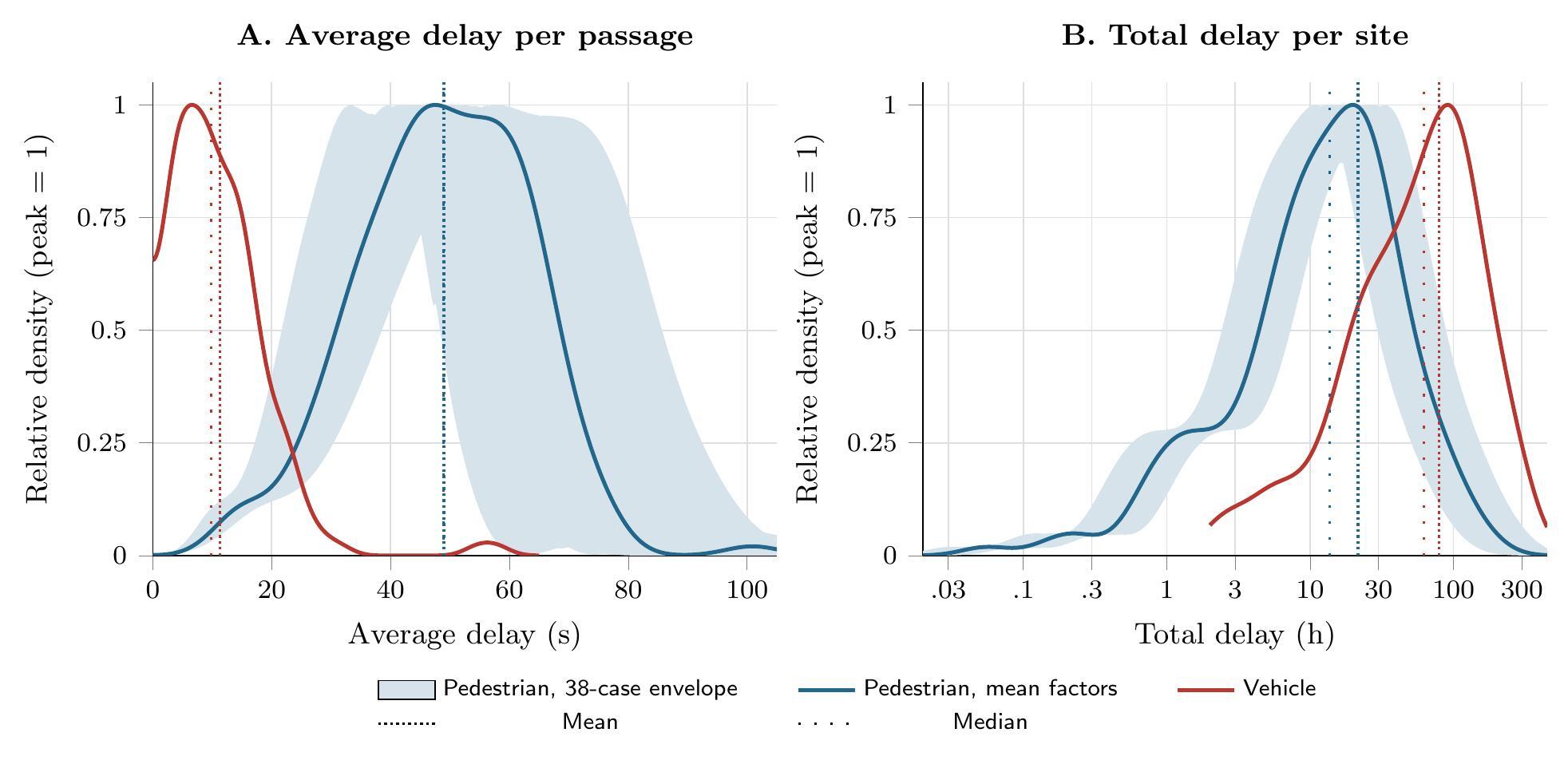
Table 1.Estimated delay under current timing and the 30-second first-call experiment. Pedestrian columns report seconds per estimated crossing and person-hours; the vehicle column reports seconds per detected vehicle and vehicle-hours. Negative changes are hours saved. The experiment uses 95 eligible sites from the 168-site current-condition sample. Its 66 vehicle-cost sites are a subset of those 95; the other 29 save time for both modes. Estimated crossings use mean factor \(\overline{\widehat{\alpha}}_N=2.203\) (central empirical range 1.417–3.138). Totals use unrounded values.
Measure Pedestrian full Walk compliance Pedestrian observed behavior Vehicle
Mean pedestrian-delay multiplier \(\left( {\overline{\widehat{\mathit{\alpha}}}}_{\mathit{D}\mathit{q}} \right)\) 2.212 1.655 –
Empirical range of \({\widehat{\mathit{\alpha}}}_{\mathit{D}\mathit{q}}\) 1.217–3.671 0.886–2.738 –
Current timing: 2,226 site-hours at 168 sites
Total delay (h) 3,632.4 2,717.1 13,279.3
Mean delay (s per passage) 39.8 29.8 10.4
Thirty-second experiment: 95 eligible sites
Current mean delay (s per passage) 38.05 28.46 9.55
Retimed mean delay (s per passage) 26.46 19.79 11.01
Change in delay, all 95 eligible sites (h) −439.70 −328.90 +885.93
Change in delay, 66 vehicle-cost sites (h) −335.96 −251.31 +1,049.25
Aggregate allocation ratio, pedestrian h saved per vehicle h added \(\left( \widehat{\mathit{R}}_{\mathit{P}\mathit{V},\mathit{q}} \right)\), 66 sites 0.320 0.240 –
Figure 1
Figure 1.Peak-normalized site distributions under full Walk compliance; each curve has maximum height one, so the panels compare shapes rather than density magnitude. Panel A shows mean pedestrian delay in seconds per estimated crossing (blue; mean 48.98, median 48.88) and mean vehicle delay per detected vehicle (red; mean 11.28, median 9.77). Panel B shows pedestrian person-hours (blue; mean 21.62, median 13.66) and vehicle-hours (red; mean 79.04, median 62.43). Dense dotted lines mark unweighted site means and loose dotted lines mark medians. The 39.8-second value in the text is the crossing-weighted network mean pedestrian delay. Each of the 38 pedestrian calibration curves is normalized separately before forming the pale-blue envelope; the aggregate average-delay ratio remains 2.685–4.788 (SI-4). Vehicle estimates do not use pedestrian calibration.

At the 95 intersections eligible for the 30-second experiment, estimated pedestrian delay under full Walk compliance falls from 38.05 to 26.46 seconds per crossing. Vehicle delay rises from 9.55 to 11.01 seconds per detected vehicle. At 29 intersections, both modes spend less time waiting: together they save 103.74 pedestrian-hours and 163.32 vehicle-hours. At the other 66 intersections, pedestrians save time while vehicles incur additional delay (Figure 2). Across all 95 intersections, the break-even pedestrian-wait weight is 2.42 under full compliance and 3.23 under observed behavior (Table 2).
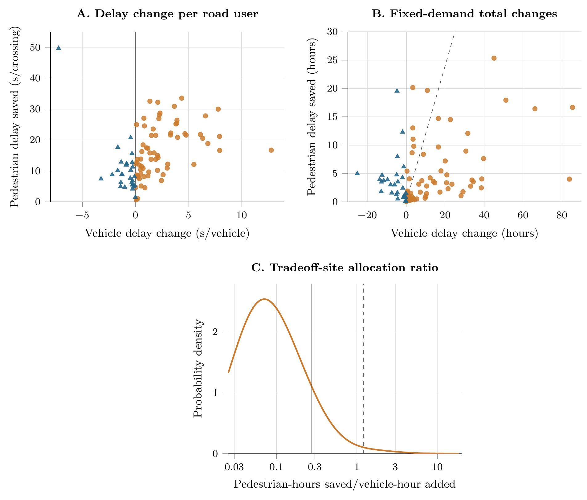
Figure 2
Figure 2.Thirty-second-cap fixed-count results using mean factors and full Walk compliance. Panel A reports seconds per estimated crossing and detected vehicle. Orange circles are the 66 vehicle-cost sites; blue triangles are the 29 sites where both modes save time. In Panel B, the dashed line is zero equal-clock-time balance at occupancy 1.2. Panel C shows pedestrian-hours saved per vehicle-hour added; the solid line is the 0.274 median and the dashed line is the equal-weight break-even value at occupancy 1.2.
Table 2.Pedestrian-wait weights \(\theta_p^*\) required for a positive aggregate balance at mean vehicle occupancy 1.2. A pedestrian minute must receive strictly more than \(\theta_p^*\) times the weight of a vehicle-occupant minute. Screened samples apply the \(\rho<0.75\) rule; “same sites” restores excluded approaches; “all eligible” also restores excluded sites. Each threshold uses all sites in its row, not the 66-site allocation ratio in Table 1. Totals are calculated from unrounded values.
Specification Cap (s) Sites \(\theta_{p}^{\ast}\), full \(\theta_{p}^{\ast}\), behavior
Screened 15 85 1.90 2.54
20 89 2.16 2.89
30 95 2.42 3.23
45 100 2.08 2.77
No screen, same sites 15 85 1.74 2.33
20 89 1.94 2.60
30 95 2.11 2.82
45 100 1.96 2.63
No screen, all eligible 15 161 4.30 5.75
20 161 4.18 5.59
30 161 3.89 5.20
45 159 3.47 4.64

The break-even weight also depends on which intersections and approaches are included. For the 30-second target, restoring excluded high-flow approaches at the same 95 intersections lowers the full-compliance weight from 2.42 to 2.11. Including all otherwise-eligible intersections then raises it to 3.89. That increase of 1.78 is nearly five times the 0.37 range across wait targets in the same-site, no-screen comparison. In these comparisons, changing the included intersections affects the break-even weight more than changing the wait target. Restored \(\rho\geq0.75\) approaches reduce estimated vehicle delay in aggregate; the additional intersections account for the larger vehicle cost. SI-7 separates these effects and reports comparisons that hold the set of intersections fixed. At an assumed occupancy of 1.4, every break-even weight would be 16.7% higher.

In the seven-day analysis, the 30-second experiment reduces pedestrian delay at 32 of 35 intersections: 18 add vehicle delay and 14 reduce delay for both modes. The remaining three have no modeled change. Twenty-two intersections retain the same direction of change in both modes on all seven days. Across the week, the experiment saves 429.12 pedestrian-hours and adds 794.32 vehicle-hours under full Walk compliance. At occupancy 1.2, pedestrian waiting must receive more than 2.22 times the weight of vehicle-occupant waiting for the weighted savings to exceed the added delay (Table 3). These 35 intersections were selected because complete inputs were available. The analysis retains high flow-to-capacity observations, where vehicle-delay estimates are less reliable because queues are not modeled.

Table 3.Seven-day fixed-count results across the 35 availability-selected sites with all required inputs, assuming full Walk compliance. The balance uses \(\theta_p=1\) and \(\omega=1.2 ; \theta_p^*\) is the pedestrian-wait weight required for break-even. Totals are calculated from unrounded values.
Cap (s) Pedestrian h saved Vehicle h changed Balance (h) \[\mathit{\theta}_{\mathit{p}}^{\ast}\] Both modes benefit (sites)
15 603.20 +1,154.71 −782.45 2.30 13
20 547.43 +1,022.65 −679.75 2.24 13
30 429.12 +794.32 −524.06 2.22 14
45 265.57 +523.59 −362.73 2.37 15

The estimated gains at the 29 one-day intersections where both modes benefit require validation against pedestrian clearance, coordination, queues, and safety constraints. The experiment isolates the effect of changing signal timing at current pedestrian and vehicle volumes. It does not estimate how people might change their route, departure time, crossing location, or travel mode in response.

Acknowledgments

Zhenyu Liu collected the manual field observations used in calibration. Keng Io Choy collected the video observations and supplied upstream pedestrian and signal tables. Anthropic Claude and OpenAI Codex assisted with code review and manuscript editing; the author verified the analysis and text.

Data and Code Availability

Analysis scripts and derived, non-identifying outputs used in the tables and sensitivity checks are provided as supplementary material with this article. Raw controller histories cannot be redistributed under the local archive terms.

Funding and Conflict of Interest

The author reports no project-specific funding or conflict of interest.

Submitted: August 21, 2026 AEST

Accepted: October 01, 2026 AEST

References

Bureau of Transport Statistics. 2014. Household Travel Survey Report: Sydney 2012/13. No. 2014/11. Transport for NSW. https:/​/​www.transport.nsw.gov.au/​sites/​default/​files/​media/​documents/​2017/​r2014-11-hts-summary-report_12-13-1.pdf.
Choy, Keng Io, and David M. Levinson. 2026. “Pedestrian Non-Compliance at Signalised Intersections in Sydney.” https:/​/​github.com/​chyy512/​PedestrianNoncomplianceAnalysis.
Karimpour, Abolfazl, Jason C. Anderson, Sirisha Kothuri, and Yao-Jan Wu. 2022. “Estimating Pedestrian Delay at Signalized Intersections Using High-Resolution Event-Based Data: A Finite Mixture Modeling Method.” Journal of Intelligent Transportation Systems 26 (5): 511–28. https:/​/​doi.org/​10.1080/​15472450.2021.1926246.
Google Scholar
Levinson, David M. 2026a. “Estimating Pedestrian Flows and Signal Delay from Sydney Traffic-Signal Event Histories.” Findings, October 20. https:/​/​doi.org/​10.32866/​001c.172160.
Google Scholar
Levinson, David M. 2026b. “Testing Pedestrian Flow and Delay Estimation from First-Actuation Latency.” Findings. https:/​/​doi.org/​10.32866/​001c.166369.
Google Scholar
Liang, Xiao (Joyce), S. Ilgin Guler, and Vikash V. Gayah. 2020. “Traffic Signal Control Optimization in a Connected Vehicle Environment Considering Pedestrians.” Transportation Research Record 2674 (10): 499–511. https:/​/​doi.org/​10.1177/​0361198120936268.
Google Scholar
Roshandeh, Ali M., Herbert S. Levinson, Zongzhi Li, Harsh Patel, and Bo Zhou. 2014. “New Methodology for Intersection Signal Timing Optimization to Simultaneously Minimize Vehicle and Pedestrian Delays.” Journal of Transportation Engineering 140 (5): 04014009. https:/​/​doi.org/​10.1061/​(ASCE)TE.1943-5436.0000658.
Google Scholar
Transport for NSW. 2024. Traffic Signal Operation. TS 05493:1.0. Transport for NSW. https:/​/​standards.transport.nsw.gov.au/​_entity/​annotation/​5c3b61e9-4ea5-ef11-b8e9-000d3a6b1b0b.
Google Scholar
Yu, Cheng, Wanjing Ma, Kun Han, and Xiaoguang Yang. 2017. “Optimization of Vehicle and Pedestrian Signals at Isolated Intersections.” Transportation Research Part B: Methodological 98: 135–53. https:/​/​doi.org/​10.1016/​j.trb.2016.12.015.
Google Scholar
Zhu, Dianchen, N. N. Sze, Zhongxiang Feng, and Ho Yin Chan. 2023. “Waiting for Signalized Crossing or Walking to Footbridge/Underpass? Examining the Effect of Weather Using Stated Choice Experiment with Panel Mixed Random Regret Minimization Approach.” Transport Policy 138: 144–69. https:/​/​doi.org/​10.1016/​j.tranpol.2023.04.020.
Google Scholar

Attachments

Powered by Scholastica, the modern academic journal management system