{gtfsrealtime}: a Package for Working with GTFS-Realtime Transit Data in R

1. Questions

The General Transit Feed Specification (GTFS) is one of the great successes of open data standards. GTFS is a standardized format for communicating transit schedule data (Voulgaris and Begwani 2023). While GTFS was originally intended to support customer-facing trip planning apps (McHugh 2013), it has seen extensive use in research (Ho 2021). Many open source tools are available for analyzing GTFS data (e.g., Herszenhut et al. 2022; Pereira et al. 2021; Reynolds et al. 2025; Kocsis and Varga 2025), many using the R statistical programming language (R Core Team 2026).

Originally, GTFS only provided data on scheduled arrival times. In 2011, GTFS-realtime was released, allowing agencies to provide real-time information (Rychev 2011). To date, most analytical applications have used the original GTFS specification (retroactively renamed GTFS-static), with some exceptions (e.g., Liu et al. 2023; Javanmard et al. 2025); a Scopus search for GTFS-realtime returns only 17 articles.^[1] One factor is the lack of tooling to read GTFS-realtime’s bespoke binary format. This article introduces the {gtfsrealtime} R package, which reads GTFS-realtime feeds into standard R data frames. It answers in the affirmative the question of whether R can be efficiently used to analyze large GTFS-realtime feeds.

2. Methods

GTFS-realtime feeds come in three types: vehicle positions, trip updates, and service alerts. The {gtfsrealtime} package exposes three functions for reading these: read_gtfsrt_positions, read_gtfsrt_trip_updates, and read_gtfsrt_alerts, which are detailed below. There are several experimental extensions to GTFS-realtime, which are not currently supported.

{gtfsrealtime} can be installed through the Comprehensive R Archive Network (CRAN):

install.packages("gtfsrealtime")

The current version is 0.2.1. {gtfsrealtime} source code and development versions are available from https://github.com/mattwigway/gtfsrealtime-r.

For performance, {gtfsrealtime} has components written in Rust (Rust Team 2025); CRAN provides binary packages for the most recent version of R on Windows and macOS (if you experience installation issues, ensure you are using the latest version of R).

Once installed, it can be loaded (along with a few other packages we will be using):

library(gtfsrealtime)
library(ggplot2) # for plotting
library(dplyr) # for general data manipulation
library(data.table) # for high-performance data filtering
library(sf) # for spatial data analysis

The following sections demonstrate the main functions of the package, using example data shipped with the package. Note that the example vehicle positions are from a different time period than the other datasets and cannot be joined with them.

read_gtfsrt_positions

Read vehicle positions with read_gtfsrt_positions. The feed used below comes from the New York City bus network. This file is included with {gtfsrealtime} and is compressed with bzip2. {gtfsrealtime} can read uncompressed files and files compressed with zip, gzip, or bzip2, from the local machine or a URL. To use with your own feed, replace VEHICLE_POSITIONS_FILE with your own file or URL.

GTFS-realtime does not include timezone information. We specify a timezone so that times are automatically converted to local time. Timezones are specified in standardized TZ database format (generally Continent/City; see list here). {sf} is an R package for geographic data (Pebesma 2018; Pebesma and Bivand 2023); specifying as_sf=TRUE will convert the data to {sf} format so it can be mapped.

VEHICLE_POSITIONS_FILE = system.file("nyc-vehicle-positions.pb.bz2",
    package = "gtfsrealtime")
positions = read_gtfsrt_positions(
    VEHICLE_POSITIONS_FILE,
    "America/New_York",
    as_sf = TRUE
)

This produces a data frame of the positions file. A few rows are shown in Table 1 (only the most relevant columns are shown; all are described in the documentation).

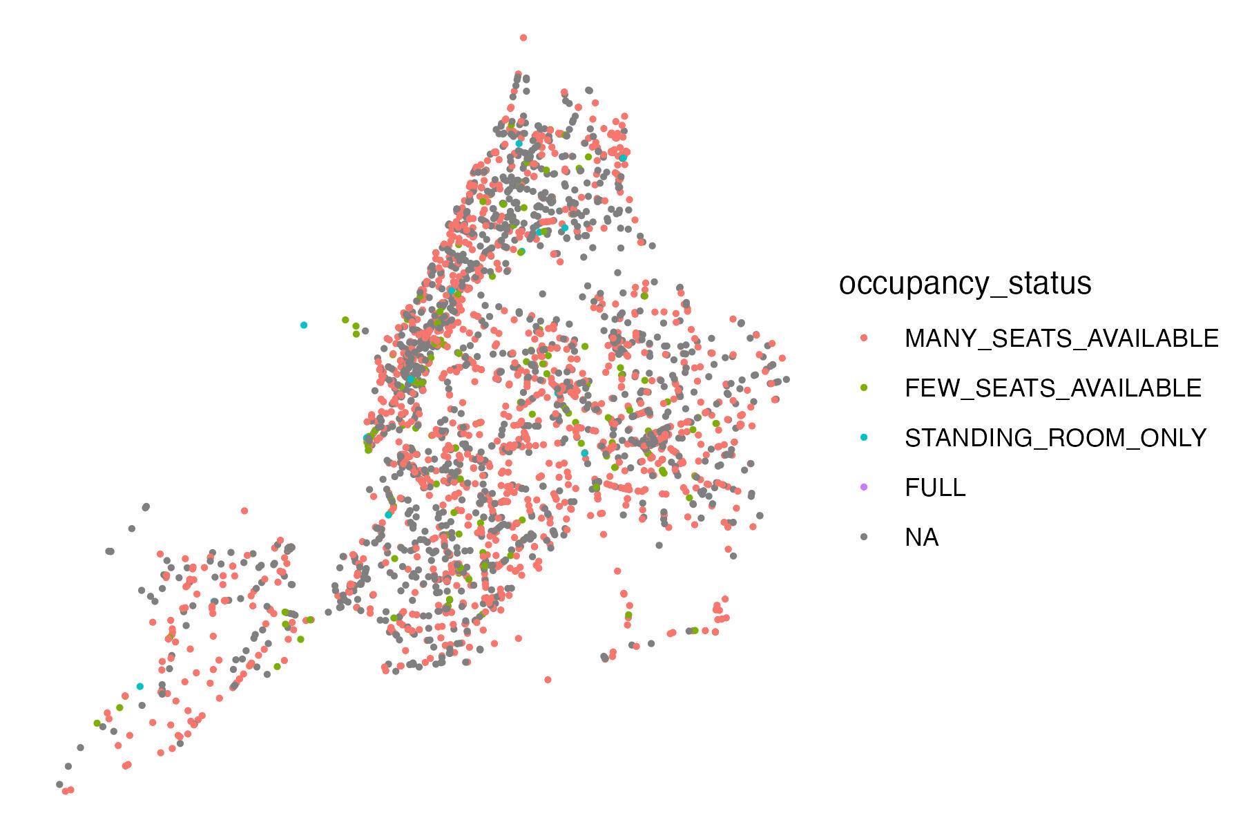
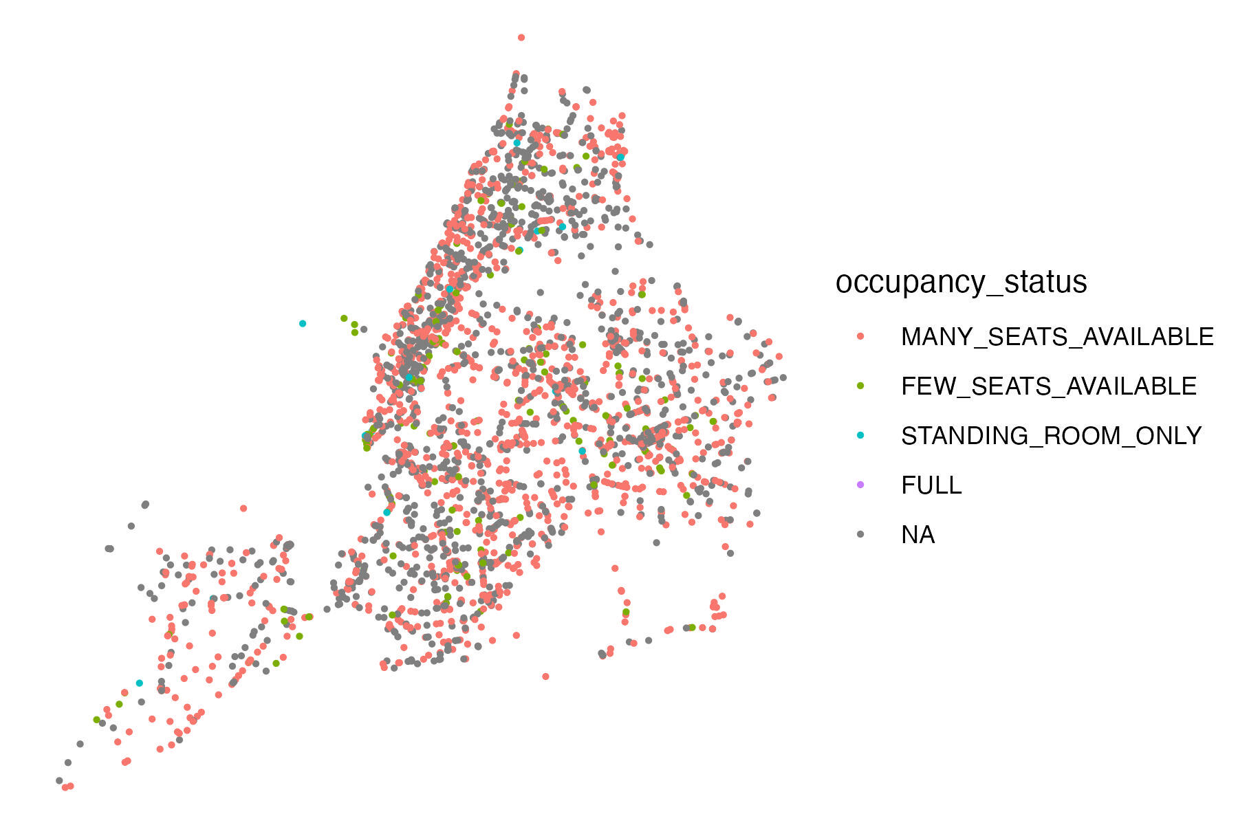
Since we read the data using as_sf=TRUE, we can also map the locations of all vehicles, colored by how full they are (Figure 1). One could use other packages such as ggspatial (Dunnington 2025) to add a basemap, scale bar, etc.; this is left to the reader for brevity.

positions |>
    ggplot(aes(color = occupancy_status)) +
    geom_sf(size = 0.5) +
    theme_void()

Figure 1.Bus positions in NYC

read_gtfsrt_trip_updates

{gtfsrealtime} likewise includes an example trip updates feed from New York MTA buses, which we can read with read_gtfsrt_trip_updates. Modify TRIP_UPDATES_FILE to work with your own file or URL.

TRIP_UPDATES_FILE = system.file("nyc-trip-updates.pb.bz2",
    package = "gtfsrealtime")
updates = read_gtfsrt_trip_updates(
    TRIP_UPDATES_FILE,
    "America/New_York"
)

GTFS-realtime trip updates are hierarchical; one trip update can contain information about the trip as a whole as well as updates for multiple stops along that trip. read_gtfsrt_trip_updates() flattens that structure into a data frame. As a result, the same id may appear in multiple rows when the feed contains stop-level updates for multiple stops. In Table 2, we inspect all rows associated with one id (and show the most relevant columns). If a trip update has no stop time updates, it will appear as a single row with all the stop-specific fields NA.

When reading this example feed, {gtfsrealtime} warns that some GTFS-realtime entity IDs are duplicated, which is problematic since these are used to identify the rows belonging to a single trip update. In these cases, the package appends suffixes such as _duplicated_1 so that each trip update can be represented with a unique id within a feed (when reading a ZIP file containing multiple feeds, ids are only unique within each of the contained feeds, which can be disambiguated with the file_index field). This deduplication applies only to the id field. Other fields, for example trip_id, are not modified so they will still correctly join with GTFS-static. Deduplication also happens with alerts and vehicle position ids.

read_gtfsrt_alerts

ALERTS_FILE = system.file("nyc-service-alerts.pb.bz2",
    package = "gtfsrealtime")

alerts = read_gtfsrt_alerts(
    ALERTS_FILE,
    "America/New_York"
)

Like trip updates, alerts are hierarchical; one alert can include multiple time periods, “informed entities” (such as routes or stops), and languages. read_gtfsrt_alerts() flattens this structure, repeating the alert for every combination of time period, entity, and language. Therefore, the same alert id may appear in multiple rows.

In Table 3, we select the first alert and display the route or stop fields and the alert text. This alert appears as two rows because it affects two routes.

Archived data

Archived data is often useful for analytical applications; {gtfsrealtime} also supports reading directly from ZIP files containing multiple GTFS-realtime feeds (for example, all vehicle positions over the course of a day). Examples of working with archived data, including vehicle position animations and stringline charts, are in the {gtfsrealtime} documentation.

3. Findings

This article has introduced the {gtfsrealtime} R package, an open-source (MIT-licensed) package for reading GTFS-realtime data into R data frames. As far as we know, this is the only actively-maintained package for reading GTFS-realtime into R. It reads the hierarchical GTFS-realtime format into a tabular format, which is conducive to efficient analysis in R. It aims to be as user-friendly as possible, handling duplicate IDs, adding factor columns rather than numeric codes for categorical variables, and processing timestamps into R date-time objects. It is fast, reading a full day of New York City vehicle positions (n=2.8 million) in 15 seconds on an M1 Macbook Pro—fast enough to readily analyze months or years of data.

We are aware of only one other actively-maintained option for reading GTFS-realtime data into R. GTFS-realtime is based on the Protocol Buffers format, and as such the {RProtoBuf} package (Eddelbuettel et al. 2016), a general-purpose package for reading any Protocol Buffers-based format, can read it. {RProtoBuf} actually reads GTFS-realtime somewhat faster than {gtfsrealtime} (the same full day of vehicle positions takes only 3 seconds to read). However, it returns data in a hierarchical format that is not conducive to efficient analysis in R. Converting to the tabular format necessary for further analysis takes an additional 24 minutes using vapply and lapply.^[2] RProtoBuf also does not provide GTFS-realtime specific features such as data compression, ID deduplication, or time zone parsing. Another package, {gtfsway}, has not been maintained in many years and is formally archived (Cooley, n.d.). There are of course also GTFS-realtime bindings in many other languages, such as Python.

There is a wealth of applications of real-time transit data—for example, accessibility analysis (e.g., Wessel and Farber 2019), operations (e.g., Aemmer et al. 2022), or passenger information evaluation (e.g, Newmark 2024). We hope that the {gtfsrealtime} package will support these types of analysis and more, and will underly development of additional standardized packages for common analyses using realtime data.