1. Questions
Induced demand is commonly described as the response of travel to lower generalized cost. Lee, Klein, and Camus define induced traffic as movement along a travel-demand curve, where price includes travel time and other user costs (Lee et al. 1999). The same demand curve has a reverse implication: if generalized cost rises, equilibrium travel should fall. Empirical studies of capacity reduction describe related outcomes as reduced, suppressed, or disappearing traffic (Goodwin et al. 1998; Cairns et al. 2002; Behrens and Kane 2004; Zhu et al. 2010).
Braess paradox supplies one network mechanism for this reverse case. Under user equilibrium, adding a link can increase travelers’ costs rather than reduce them (Braess 1968; Braess et al. 2005; Murchland 1970; Yang and Bell 1998). Prior work gives tests for equilibrium cost changes under demand changes and added routes (Dafermos and Nagurney 1984), shows that the paradox can disappear at higher demand when the Braess link is no longer used (Nagurney 2010), and examines elastic-demand traffic paradoxes (Hallefjord et al. 1994; Tu et al. 2019; Nagurney and Nagurney 2020). Related network and demand paradoxes also appear in the Downs–Thomson/Pigou–Knight–Downs tradition and in empirical induced-demand and road-capacity literatures (Downs 1962; Thomson 1977; Pigou 1920; Knight 1924; Hansen and Huang 1997; Noland 2025).
This note connects those strands by making one sign implication explicit and by mapping where the Braess cost increase occurs in Braess’s original numerical network. The contribution is conceptual and classificatory, not a general network-design theorem. With a strictly decreasing inverse-demand curve, reduced demand follows once the added link raises equilibrium cost. The point of the sweep is therefore to map where that premise holds. I ask: where, in the original Braess network with downward-sloping inverse demand, does the added link raise equilibrium cost?
2. Methods
The model is Braess’s original directed four-node network with one origin-destination pair (Braess 1968; Braess et al. 2005). This numerical example is the case repeated in early discussions of the paradox (Murchland 1970; Frank 1981; Pas and Principio 1997). The topology is also a minimal critical topology used to analyze the magnitude of Braess penalties (Penchina 1997). Link 1 runs from Origin to Upper, link 3 from Upper to Destination, link 2 from Origin to Lower, and link 4 from Lower to Destination. Link 5 is the candidate Upper-to-Lower connector. The upper path is links 1–3, the lower path is links 2–4, and the added-link path is links 1–5–4. The link performance functions are:
\[\small t_1(x)=10x,\quad t_4(x)=10x,\quad t_2(x)=50+x,\quad t_3(x)=50+x,\quad t_5(x)=10+x,\] with fixed demand The candidate link is solved both off and on.
For each scenario, the model enumerates all simple origin-destination paths and solves static Wardrop user equilibrium by Method of Successive Averages (Sheffi 1985). At each iteration, link costs are evaluated from current flows, all demand is assigned to the current shortest path, and path flows are averaged using the diminishing step size This averaging is the convergence device: it damps path switching. The stopping tolerance is after at least five iterations, with a 120-iteration maximum. For the nonnegative affine and Bureau of Public Roads-style separable link costs used here, this is the standard monotone user-equilibrium setting.
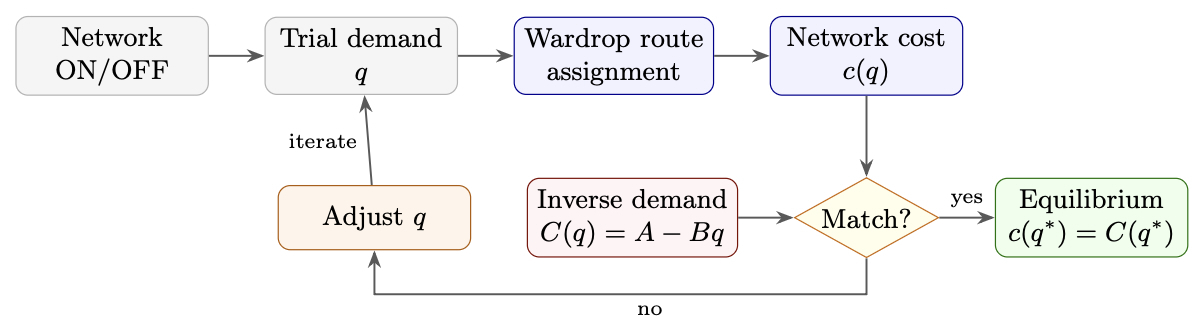
Elastic demand uses inverse demand \[C(q)=A-Bq.\] The default elastic case sets and so the zero-cost demand intercept remains Computationally, the model uses an outer bisection on for each trial quantity, it solves Wardrop equilibrium and compares the resulting network cost with Bisection is appropriate when is monotone over the bracket, as it is for the downward-sloping inverse demand and monotone link costs used in the reported sweeps. Reported elastic costs are network costs they equal at the exact fixed point, apart from numerical tolerance and rounding. Conceptually, the elastic-demand solution is a fixed point where route flows and demand agree simultaneously: (Fig. 1). Here is the network-side equilibrium cost relation, and is the demand-side willingness-to-pay relation.

Proposition. For scenario elastic equilibrium satisfies If is strictly decreasing and the added link raises elastic equilibrium cost, then Reduced demand is therefore the logical implication when Braess’s paradox raises equilibrium cost under this demand specification. Cells classified as “demand unchanged” are numerical-tolerance or unused-link boundary cases, not a separate behavioral outcome.
The interest is therefore not the sign of the demand response, which follows once equilibrium cost rises. The interest is where the added link raises equilibrium cost in the first place.
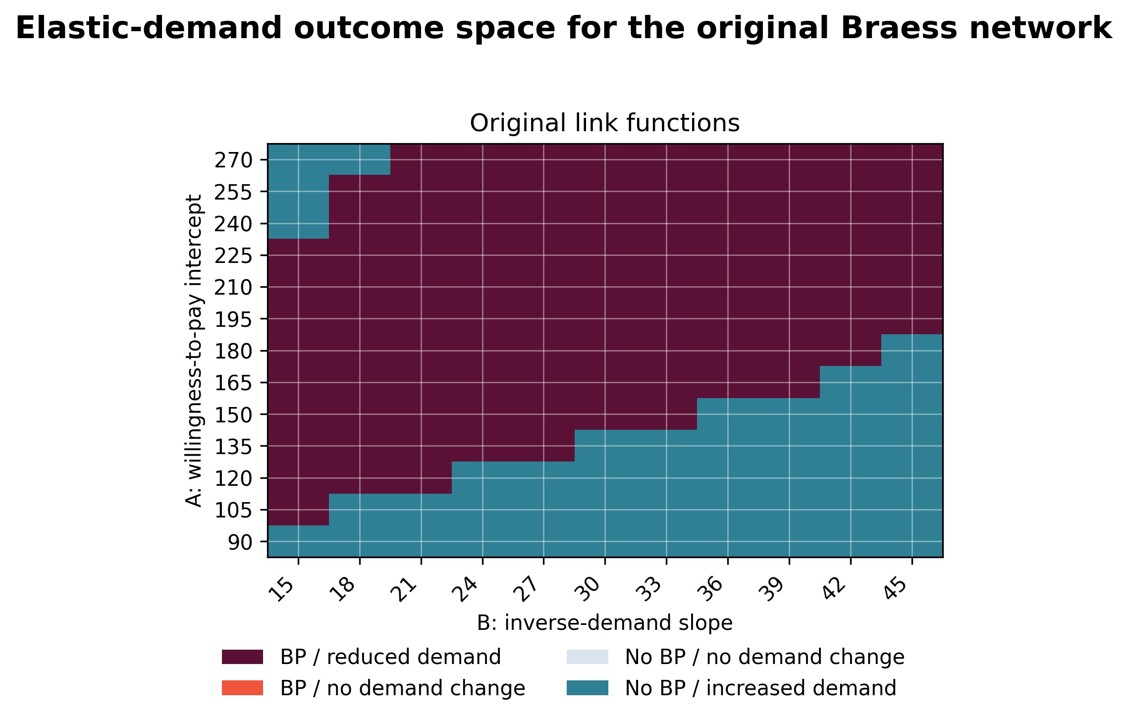
The Braess flag is The reported sweep varies and over 13 by 11 evenly spaced grid values, for 143 grid points, while holding Braess’s original link functions fixed. The numerical results were generated in the browser implementation described in the Data Availability section.
3. Findings
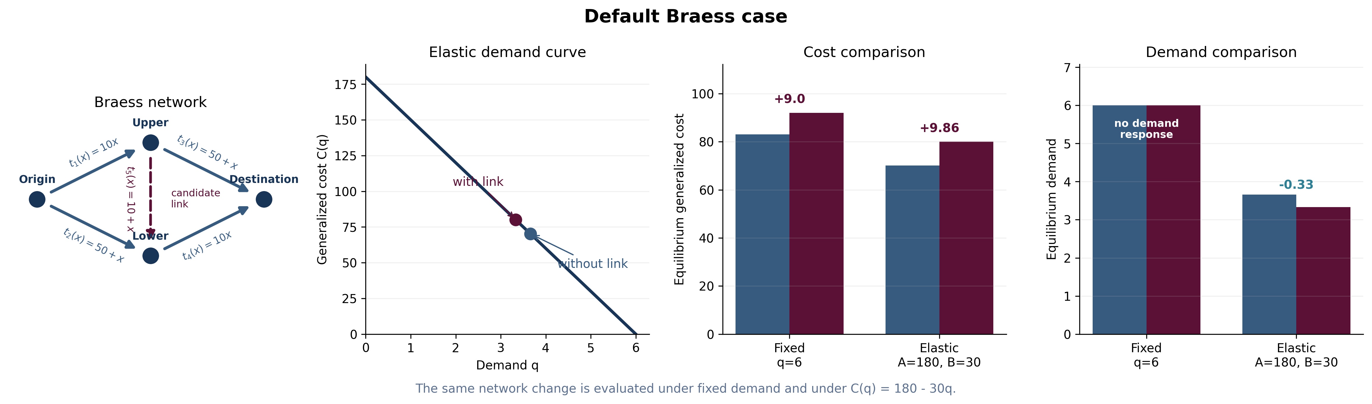
The fixed-demand default reproduces the original Braess paradox. Without the added link, equilibrium cost is 83.00. With the added link, equilibrium cost is 92.00, a 9.00-unit increase. Total travel time rises from 498.00 to 552.00.
The elastic-demand default converts the same network effect into reduced demand. With and the added link raises equilibrium cost from 70.14 to 80.00 and lowers equilibrium demand from 3.66 to 3.33 (Fig. 2). The result is the induced-demand comparative static with the network-cost sign reversed: the added link changes the network equilibrium cost relation, and demand adjusts until generalized cost equals willingness to pay.

The outcome-space sweep is descriptive rather than inferential: it locates the Braess region in the reported A-B grid. In that grid, the added link raises equilibrium cost in 97 of 143 cells (67.8%), and demand is lower in every one of those cells. Where the added link does not raise cost, demand increases in all 46 cells. The two sign-inconsistent cases under a downward-sloping inverse-demand curve, Braess with increased demand and no Braess with reduced demand, have zero grid points (Fig. 3).

The outcome map gives a compact diagnostic for interpreting added links under elastic demand. The “No BP / increased demand” class is the familiar induced-demand case: the added link does not worsen equilibrium cost and demand increases. The “BP / reduced demand” class is the reverse case: the added link worsens equilibrium cost through Braess paradox and demand falls. The same inverse-demand relation appears in both regions; the network determines whether the added link lowers equilibrium cost and induces demand or raises equilibrium cost and reduces demand.
Data Availability
The Braess Explorer app, model code, export scripts, CSV files, and figures are at https://github.com/dlevinson/braess-js. The app runs in the browser from https://transportlab.sydney.edu.au/wp-content/uploads/braess/documentation.html.
AI Acknowledgment
The author used OpenAI ChatGPT/Codex as an editorial and computational assistant during writing and revision, for figure styling, replication-package organization, and drafting support. The author reviewed, verified, and takes full responsibility for all analyses, interpretations, text, figures, and submitted materials.