
1. Questions
Logistic curves are widely used to describe growth and diffusion in biology, infrastructure, and technology studies (Rogers 2003; Marchetti and Nakicenovic 1979; Nakicenovic and Grubler 1991; Grubler and Nakicenovic 1991; Meyer et al. 1999; Meade and Islam 2006; Garrison and Levinson 2014). In the technology-diffusion literature, a common summary is the midpoint together with a duration measure, usually the time from 10% to 90% of the asymptote (Marchetti and Nakicenovic 1979; Nakicenovic and Grubler 1991; Grubler and Nakicenovic 1991; Meyer et al. 1999; Bento and Wilson 2016). In other settings, authors use tangent constructions or higher-derivative characteristic points to identify transitions (knees of the curve) from birth to rapid growth, and from rapid growth toward saturation (Passos et al. 2012; Rzadkowski et al. 2014).
Stage-transition rules for sigmoid curves can be classified by the mathematical object they use. Convention-based rules select fixed percentiles or fixed offsets from the midpoint. Shape-based rules use derivatives or geometric curvature of the fitted curve. Estimator-based rules infer breakpoints from piecewise regressions, splines, or statistical stopping criteria. Decision-based rules use a stopping criterion rather than a geometric landmark. These families can yield similar dates in some settings, but they are conceptually distinct because they optimise or threshold different quantities.
This note brings several familiar rules into one common form to make their relationship transparent. The goal is not to introduce a new estimator. It is to show that several stage-transition rules used for the standard logistic are equivalent to choosing different percentile windows on a standardised time scale.
2. Methods
The analytic rules considered here represent two common ways of defining transition dates, namely a derivative-based rule and a geometric construction, while the percentile conventions provide explicit reference windows for comparison. Appendix A places these within a broader taxonomy, and Appendix B gives the algebra for the closed-form constants.
Consider the standard logistic function
y(t)=K1+exp[−b(t−t0)],
where is the asymptote, is the growth-rate parameter, and is the inflection date. Define the standardised time coordinate
z=b(t−t0),
and the normalised level
p(z)=y(t)K=11+e−z.
For the standard logistic, any symmetric stage-transition rule can be written as
tL=t0−cb,tR=t0+cb,
where is a rule-specific constant on the standardised time scale. The corresponding right-side level is
p=11+e−c,
so the full symmetric percentile window is
(1−p, p).
This re-expression is useful because it places different transition conventions on the same scale. Once written in this form, apparently different symmetric rules differ only in the constant and therefore in the implied central percentile window of the asymptote
The closed-form rules considered here are as follows.
Third-derivative rule
This rule identifies the two symmetric dates at which the third derivative of the logistic is zero. For the standard logistic, that yields
cy‴=ln(2+√3)≈1.317,
which corresponds to the percentile window 21.13% to 78.87% of
Tangent-at-inflection rule
This rule draws the tangent line at the inflection point and uses its intersections with the lower and upper asymptotes to define the transition dates. For the standard logistic, this gives
ctan=2,
which corresponds to the percentile window 11.92% to 88.08% of
Percentile conventions
The standard diffusion-duration convention defines the transition window as the period between 10% and 90% of giving
c10-90=ln(0.90.1)≈2.197.
Similarly, the commonly used 15% to 85% window implies
c15-85=ln(0.850.15)≈1.735.
These percentile conventions are included as explicit reference points for comparison with the derivative-based and tangent-based rules.
Illustrative fitted benchmark
To compare these fixed conventions with an estimated breakpoint method, consider the continuous three-segment linear model
ˆy(t)=α+β1t+β2max
This hinge specification imposes continuity at both breakpoints. The estimated breakpoints are chosen by least squares. Unlike the closed-form rules above, this fitted benchmark does not imply a universal constant in Its breakpoints depend on the fitting window, weighting, observation grid, and model specification.
For transparency, the comparison uses one exact synthetic logistic example with and observed on the symmetric window at intervals of 0.25 time units. The value of does not affect the breakpoint dates and is chosen arbitrarily. Candidate breakpoints are restricted to the observation grid and to specifications leaving at least 10% of observations in each segment. For each candidate pair, coefficients are estimated by ordinary least squares using the hinge basis above. The reported breakpoints are the pair that minimise the residual sum of squares. The calculation was carried out in Python using a brute-force search with numpy.linalg.lstsq. The script used to generate the synthetic example, estimate the free segmented-regression breakpoints, and reproduce Figure 1 is provided in the Appendix.
3. Findings
Figure 1 shows that the segmented-regression breakpoints lie very close to the tangent-at-inflection dates and farther from the third-derivative dates. The estimated breakpoints are 2006.36 and 2017.61, compared with 2006.29 and 2017.71 for the tangent rule, 2007.04 and 2016.96 for the 15% to 85% benchmark, and 2008.24 and 2015.76 for the third-derivative rule. For estimation, the segmented fit is left unconstrained, so the fitted piecewise-linear approximation can fall slightly below zero near the edge of the fitting window, or above even though the logistic curve itself remains bounded between 0 and
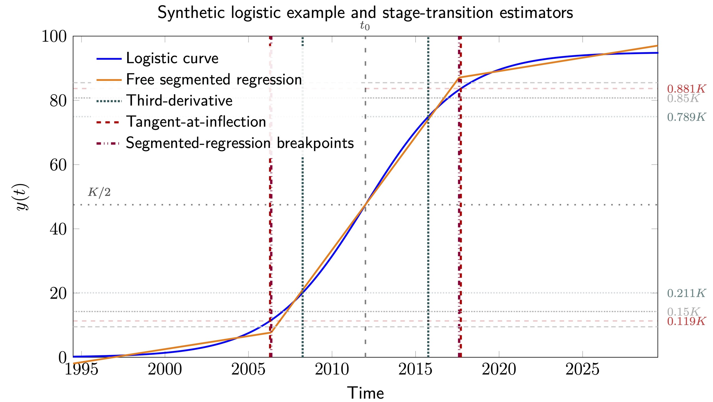
The main result is a compact unification. The common analytic stage-transition rules for the standard logistic differ only by the constant in Table 2 reports the implied percentile windows and widths.
This yields the exact ordering
\ln(2+\sqrt{3}) < \ln(0.85/0.15) < 2 < \ln(0.90/0.10),\tag{12}
that is, approximately
1.317 < 1.735 < 2.000 < 2.197.\tag{13}
Accordingly, the third-derivative rule defines the narrowest central transition window of the four rules shown here, the 15% to 85% benchmark is wider, the tangent rule wider again, and the 10% to 90% diffusion-duration measure wider still.
A second implication is interpretive. Rules that are often motivated in different ways are analytically equivalent once written on the standardised time axis. The third-derivative rule can be read as an implicit 21.13% to 78.87% convention. The tangent rule can be read as an implicit 11.92% to 88.08% convention. The 10% to 90% diffusion duration, widely used in the technology-substitution literature, is simply another member of the same family (Marchetti and Nakicenovic 1979; Nakicenovic and Grubler 1991; Grubler and Nakicenovic 1991; Meyer et al. 1999).
For the synthetic logistic described in the Methods section, the estimated segmented-regression breakpoints are 2006.36 and 2017.61. These are very close to the tangent-at-inflection dates, 2006.29 and 2017.71, and farther from the 15% to 85% dates, 2007.04 and 2016.96, and from the third-derivative dates, 2008.24 and 2015.76. In this exact-logistic example, the free segmented fit therefore behaves much like the tangent rule. This pattern is also geometrically intuitive, because the tangent-at-inflection construction gives the best local linear approximation at the point of maximum slope, so a piecewise-linear fit to an exact logistic can be expected to gravitate toward it.
A third implication concerns terminology. In diffusion studies, authors often discuss phases such as emergence, rapid growth, and maturity (Rogers 2003; Meade and Islam 2006). But the exact dates of the phase boundaries are usually not theory-implied. They are convention-implied. For the standard logistic, choosing a stage-transition rule is equivalent to choosing a percentile window, whether that choice is made explicitly, as in 10% to 90%, or implicitly, as in the tangent and third-derivative rules. The 15% to 85% benchmark is useful for comparison because it lies between the third-derivative and tangent rules, but it remains a heuristic reference point.
Authors using logistic curves should state their transition convention directly to make comparisons across studies easier and reduce the risk that different percentile conventions are mistaken for substantive disagreement about the underlying diffusion process.
AI Acknowledgment
The author used OpenAI ChatGPT/Codex as an editorial and computational assistant during writing and revision, for figure styling, and drafting support. The author reviewed, verified, and takes full responsibility for all analyses, interpretations, text, figures, and submitted materials.