

1. Questions
Commuting time is a key indicator of the spatial mismatch between residential and employment locations, which serves as a determinant of individual quality of life and the effectiveness of urban transport policies. A substantial body of research has examined how physical and environmental factors—such as population density, residential location, and car ownership—affect commuting time (Giuliano and Narayan 2003; Sohn 2005; Redmond and Mokhtarian 2001). As the field evolved, subsequent studies began to incorporate socioeconomic dimensions, exploring the relationships between commuting time, household decision-making, and wage levels (Plaut 2006; Gutiérrez-i-Puigarnau and van Ommeren 2010). Recent studies have expanded to include the psychological and subjective aspects of commuting by investigating its associations with life satisfaction and well-being (Ye and Titheridge 2017; De Vos et al. 2022). These studies have advanced our understanding of commuting behavior, yet they largely rely on static cross-sectional data that may fail to capture the dynamic variability in daily travel patterns.
Most studies on commuting time have relied on one-day travel diaries or annual travel surveys, which implicitly assume that a single observation can represent an individual’s typical travel behavior. In reality, however, commuting time is influenced by a range of external factors—including the day of the week, season, weather conditions, and traffic congestion—that generate substantial daily variability. Consequently, single-day or single-year observations may not fully capture the temporal volatility of certain determinants, suggesting a need for caution when interpreting these as stable structural relationships (Stopher et al. 2007; Goodwin 2012). Against this backdrop, this study explores the dynamic and time-varying nature of commuting behavior to provide a cautionary perspective on relying solely on single-point data.
2. Methods
This study uses driving trajectory data from electric vehicles collected by the Korea Electric Power Corporation (KEPCO). The empirical analysis in this study is based on a longitudinal dataset of time-series driving logs collected from 467 vehicles over a one-year period, from March 1, 2023, to February 29, 2024. Each vehicle was equipped with an On-Board Diagnostics (OBD) device that recorded high-resolution telematics data—including GPS coordinates, Battery Management System (BMS) metrics, and ignition status (ON/OFF)—at approximately 5-second intervals. To transform the raw telemetry into discrete analytical units, individual trips were reconstructed by defining a trip termination threshold of five minutes of continuous inactivity. Furthermore, to maintain the consistency of the annual analysis, any vehicle with missing observations during the 12-month study period was excluded from the initial dataset. To capture the dynamic shifts in commuting destinations for each vehicle, this study applied the Density-Based Spatial Clustering of Applications with Noise (DBSCAN) algorithm. Unlike centroid-based methods such as K-means, DBSCAN offers the distinct advantage of identifying clusters without a predefined number of clusters (k) and effectively filtering out “noise,” such as incidental or transient stops. By spatially clustering the primary stay points for each vehicle, the monthly occupancy rate for each cluster was calculated. A cluster was defined as the Primary Commuting Destination for a specific month if its occupancy rate reached 0.7 or higher. The temporal evolution of these dominant clusters allowed for the classification of commuting behaviors: instances where the dominant cluster remained consistent were classified as stable patterns, while instances where a dominant cluster transitioned at a specific point were interpreted as shifts in the primary life-sphere resulting from relocation or a change in employment. To ensure the statistical reliability of the findings, a final filtering process excluded vehicles with fewer than 50 valid commuting days per year, resulting in a finalized sample of 166 vehicles for the empirical analysis.
In addition, to investigate the impact of weather conditions on the daily variability of commuting times, this study utilized daily observational data provided by the Automated Surface Observing System (ASOS) of the Korea Meteorological Administration. To mitigate potential data gaps and statistical bias arising from the uneven spatial distribution of weather stations, Ordinary Kriging, a spatial interpolation technique, was applied. The data construction procedure was as follows: First, the centroids of each administrative district were extracted using spatial data from Statistics Korea. Subsequently, independent Kriging interpolations were performed for each date to transform station-based point data into administrative district-level area data, thereby constructing a comprehensive meteorological panel. For the empirical analysis, variables such as average temperature, daily precipitation, and maximum fresh snow depth were log-transformed. These regional-level explanatory variables were then merged with individual vehicle driving logs to serve as independent variables. Furthermore, to control the impact of traffic accidents on commuting time variability, daily accident statistics at the administrative district level were obtained from the Traffic Accident Analysis System (TAAS). Variables including accident dates, locations, frequency, and severity were extracted and aggregated by district and date, then integrated with the driving logs and the meteorological panel data.
To investigate the temporal variability of commuting time determinants, this study employs a State-Space Model. In this framework, regression coefficients are not assumed to be fixed constants but are instead treated as state variables that evolve over time. Unlike conventional linear regression models, the State-Space Model allows for the simultaneous estimation of both observable data and the dynamic transitions of unobservable parameters by decoupling the analysis into an Observation Equation and a State Equation.
The observation equation is expressed as follows:
yi,t=X′i,tβt+∈i,t, ∈t ∼ N(0,R)
Where is the commute time for trip i at time t, and is the observation variance representing the random error not accounted for by the model.
The state equation is expressed as follows:
βt=βt−1+ηt, ηt ∼ N(0,Q)
The term represents the state transition error, and Q is the state variance matrix that determines the temporal variability of each coefficient. If the state variance of a specific variable converges to zero, the coefficient is treated as a constant that remains stable over time. Conversely, if the state variance is significantly greater than zero, it indicates that the influence of the corresponding factor undergoes temporal transitions, reflecting its dynamic nature.
3. Findings
3.1. Estimation Results of the State-Space Model
In contrast to previous studies that estimated commuting time determinants as fixed constants using single-point cross-sectional data, this study employs a State-Space Model utilizing the Kalman Filter to capture the dynamic transitions of these determinants. The estimation results yielded an AIC of 202,108.036 and a log-likelihood of -101,031.018, providing a baseline for the statistical fitness of the model. In the observation equation, the estimated observation variance was 331.43. This indicates that the model effectively isolated the stochastic noise occurring at the individual trip level. Consequently, the proposed model successfully extracted the state variables, which represent the pure behavioral influence of the independent variables by decoupling them from transient errors.
The estimation of state variance, a core indicator of this study, empirically confirms the time-varying nature of commuting time determinants. While structural factors (e.g., departure time) showed remarkable stability, significant volatility was observed in specific exogenous factors (e.g., weather and battery status). The average regression coefficients and the corresponding time-varying characteristics for each variable are shown in Table 1.
First, departure time and arrival delay were identified as significant factors influencing commuting time. The commuting time significantly decreased for departures after the morning peak (8–9 AM, b = -23.318) and during the subsequent afternoon and evening periods (9 AM–12 AM, b = -48.440). Conversely, arrival delay situations led to a time increase of approximately 30.23 minutes. Furthermore, the state variances for these variables showed negligible estimated state variance, implying that the influence of trip patterns based on specific schedules remains largely invariant despite changes in the external environment.
Individual demographic and socio-economic characteristics showed marginal associations with commuting time. Specifically, manufacturing workers showed a decrease of approximately 14.14 minutes, while individuals in their 40s exhibited a tendency toward a 5.20-minute increase. Despite these significant impacts, the state variances for these variables remained remarkably low. This indicates that the effect of socio-economic status on commuting behavior maintains temporal stability, remaining resilient against transient exogenous noise or short-term situational fluctuations.
The stability of structural factors, such as departure time and socio-economic status, reflects the fixed nature of individuals’ long-term routines and life-spheres, which remain resilient to daily fluctuations. In contrast, the high state variance observed in weather conditions and battery status indicates that these factors are situational stressors that require immediate, short-term behavioral adjustments.
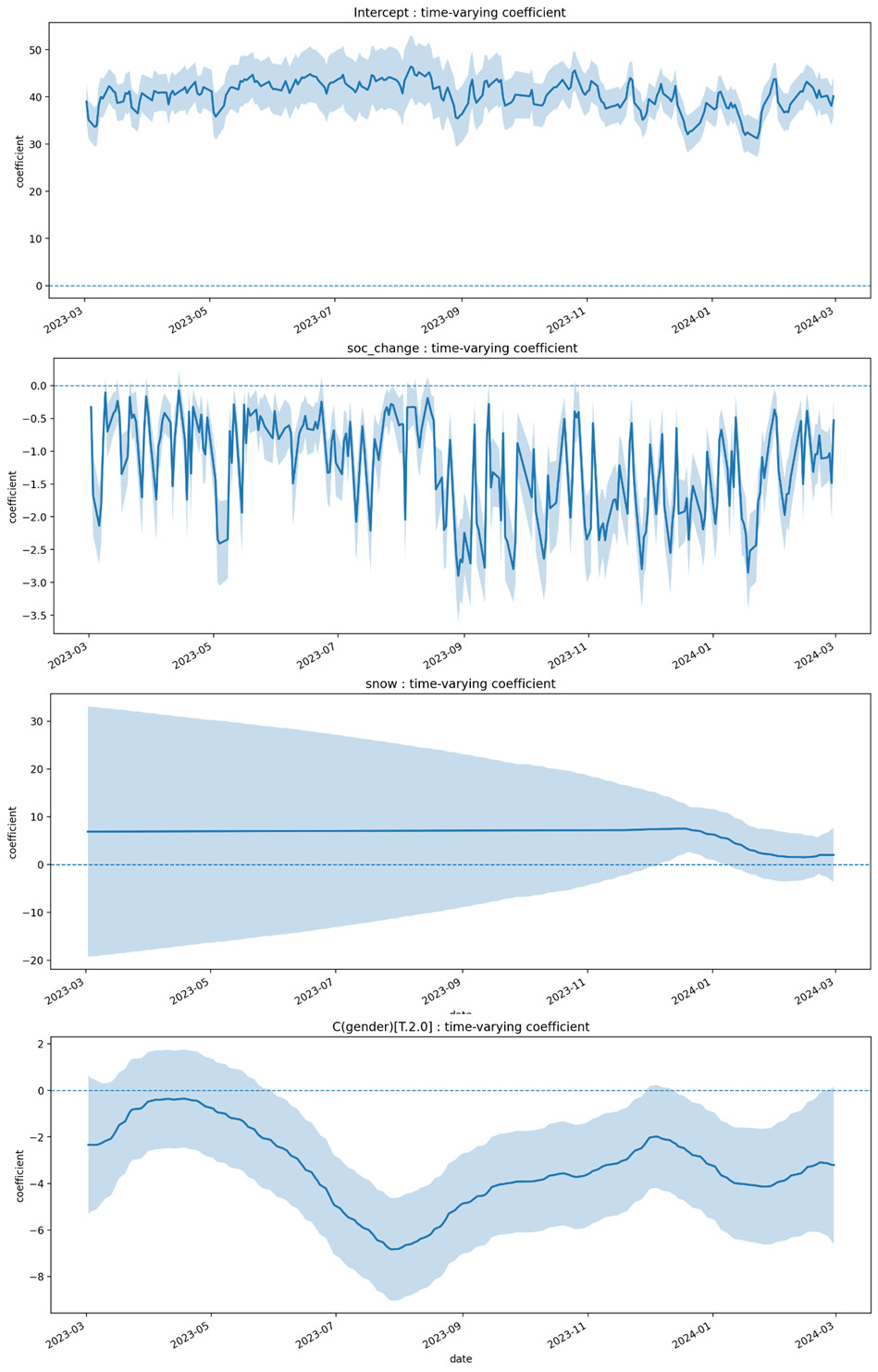
In contrast, weather conditions and the vehicle’s energy state exhibited dynamic variability. The snowfall variable (Snow) had a positive effect on commuting time (b = 6.369) with a state variance of 0.8912. This indicates that the impact of snow on commuting time is not fixed, which reflects a dynamic variability that fluctuates non-linearly depending on situational contexts, such as the amount of accumulation or the level of road clearance operations. Additionally, the State of Charge (SOC) showed a negative effect (b = -1.235) with a high state variance (0.5754). This suggests that the influence of the vehicle’s battery status on driver behavior is not constant but is instead a time-varying attribute that changes depending on the specific point in time.
Finally, the model’s intercept recorded a coefficient of 40.478 along with a high state variance of 5.5486. This indicates that even in the absence of exogenous shocks, the expected value of the baseline travel environment does not remain constant but undergoes a continuous drift. This intercept drift suggests that the baseline commuting environment is subject to unobserved temporal variations, such as seasonal shifts in traffic demand, evolving network conditions, or collective behavioral adaptation among EV users. While the model does not explicitly resolve these factors, the high state variance of the intercept captures this underlying environmental ambiguity. Ultimately, these results provide empirical evidence that the determination of commuting behavior is being constantly reconstituted according to the situational context.
These results demonstrate that the underlying baseline effects determining commuting time are in a state of constant flux over time. Consequently, while traditional cross-sectional approaches remain valuable for identifying long-term structural trends, they run the risk of overgeneralizing transient situational effects as permanent determinants in contexts with high behavioral volatility. The temporal variability of the coefficients identified in this study suggests that conventional analytical frameworks, which assume fixed constants, have overlooked the behavioral variability inherent in real-world phenomena.
3.2. Daily variability in t-statistics
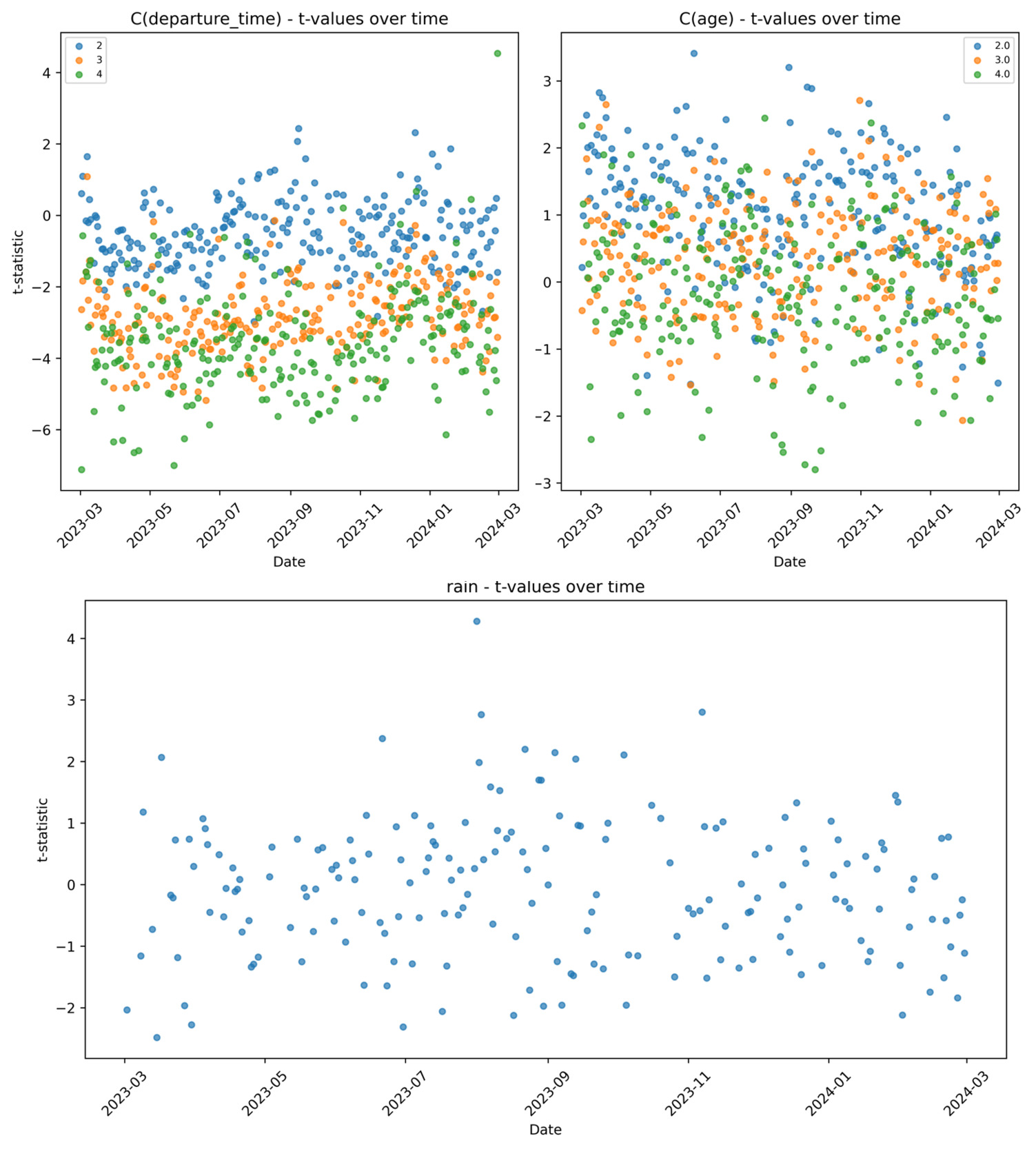
To determine whether key variables, such as age, departure time, and rainfall, maintained temporal consistency, the time-series distributions of their t-statistics were examined across daily regression models. For age-related variables, standard errors reflecting estimation uncertainty for the 40+ age group showed substantial day-to-day fluctuations. Statistical significance (|t| > 1.96) occurs on only a limited subset of days within the full analysis period. This pattern suggests that although age-based differences in commuting time exist, their effects lack sufficient magnitude relative to daily traffic conditions or demand variations, rendering consistent statistical significance difficult to establish in daily analysis.
In contrast, departure time variables exhibited both statistical significance and stability. Groups departing later than the reference time consistently displayed large negative t-statistics, ranging from -2 to -6 over extended periods. This confirms that avoiding peak congestion hours reliably shortens commuting duration across all external environmental variations. Ultimately, departure timing exerts a greater influence than daily-fluctuating environmental factors, thereby establishing it as the most stable determinant of commuting time.
Rainfall exhibited highly unstable statistical patterns. Its t-statistics fluctuated widely between -3 and +4 across dates, with both coefficient signs and magnitudes varying inconsistently. This indicates that the short-term effects of precipitation on commuting time are not fixed parameters but emerge locally on specific days through interactions with rainfall intensity, timing, traffic incidents, and demand conditions.
3.3. Discussion
Through the application of a state-space model, this study confirmed that while commuting schedules remain relatively stable, exogenous factors such as weather conditions and battery status exhibit short-term and localized characteristics, with their signs and magnitudes fluctuating sharply depending on the specific point in time. These findings indicate that determinants of commuting time are not fixed constants, which instead exhibit time-varying properties that dynamically respond to situational contexts. Consequently, the conventional assumption of coefficient invariance—reliant on single-day data—may diverge substantially from actual behavioral dynamics.
Methodologically, this study cautions that single-point survey designs risk misinterpreting transient noise as structural relationships, which emphasizes the need for more advanced approaches, such as state-space models or dynamic estimation techniques, in future studies. From a policy perspective, the findings support a shift away from static designs predicated on an ‘average commuter’ toward context-aware policy design that accounts for time-of-day and date-specific environmental variations, while establishing dynamic evaluation frameworks to track long-term policy responses.
In addition, it is important to note that these findings are based on a filtered sample of EV users in South Korea whose commuting patterns were inferred via telematics data. Therefore, the extent of coefficient instability observed here may vary for other transportation modes or demographic groups, and these results should not be interpreted as a general proof that all annual cross-sectional analyses are invalid.
In summary, this study empirically supports Goodwin’s (2012) argument that only longitudinal analysis tracking the same individuals’ behavioral changes can accurately capture behavioral volatility and transition processes. By demonstrating the risk of overstating behavioral stability in one-day cross-sectional analyses, this research provides evidence that in contexts with high behavioral volatility, transportation analysis should incorporate greater sensitivity to temporal shifts.