Spatial Dependency Patterns in Weather-Enhanced Bike-Share Demand Forecasting in Washington DC

1. Questions

Every day, shared bicycles accumulate at popular destinations at offices, metro stations, and shopping areas while other docking bays sit empty. To restore balance, operators move bikes by van in a costly process called rebalancing (Fukushige et al. 2022). Effective rebalancing requires anticipating demand before shortages arise. Convolutional Long Short-Term Memory (ConvLSTM) networks, which analyze temporal and spatial patterns simultaneously, have demonstrated strong performance in bike-share demand forecasting (He and Shin 2020; Tang et al. 2024). Yet these models typically do not reveal which zones most strongly influence demand elsewhere, leaving operators uncertain where to prioritize rebalancing.

A standard planning assumption holds that nearby zones influence each other more than distant ones (Tobler 1970). Miao et al. (2025) tested this assumption in New York City by applying SHAP (SHapley Additive exPlanations) to December 2023 Citi Bike data on member and casual bikers. Members are routine commuters with predictable patterns, while casual users make irregular, leisure-oriented trips with dispersed demand (Lee and Kim 2022; Wang et al. 2024). They found that spatial influence was directional, exhibited no distance decay, and that casual riders showed far weaker zone-to-zone coupling than annual members. Previous studies have largely overlooked weather variables in spatial demand models, an omission that may introduce significant prediction errors, particularly in winter months when weather strongly affects ridership.

We replicated and extended these findings to Washington, D.C.—a structurally distinct city with a federal employment core, extensive Metro network, and commuter-cycling culture. We also employed permutation-based perturbation, a computationally simpler alternative to SHAP that similarly measures how removing a zone’s signal affects predictions. January represents DC’s coldest month (average ≈ 2 °C), making weather a stronger demand driver than in warmer periods (Bean et al. 2021; Gebhart and Noland 2014). Three questions guide this study:

Q1. Do spatial influence patterns in DC’s bike-share network follow geographic proximity?

Q2. Do member and casual users show distinct dependency structures?

Q3. Does adding weather and temporal data improve forecast accuracy?

2. Methods

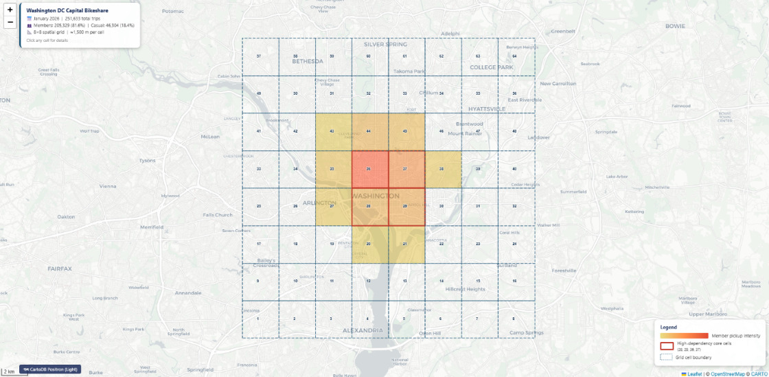
Data. We obtained all January 2026 Capital Bikeshare trip records from the operator’s open-data portal (https://capitalbikeshare.com/system-data). Of 253,418 raw records, we excluded 1,098 trips under one minute (accidental undocking), 687 trips exceeding 12 hours (unreturned bikes; current pricing charges members after 45 minutes, rendering 12-hour records operationally invalid), and records with missing coordinates. This yielded 251,633 valid trips: 205,329 by members (81.6%) and 46,304 by casual users (18.4%). Sensitivity tests using 4-hour and 6-hour maximum-duration thresholds produced virtually identical results (Supplemental Table S1). Hourly weather data—temperature, precipitation, wind speed, and humidity—were retrieved from the Open-Meteo Historical Weather Archive (https://open-meteo.com/en/docs/historical-weather-api) for the DC centroid (38.9° N, 77.03° W). Because observations were hourly, each weather vector was assigned unchanged to both 30-minute steps within its hour, precluding capture of sub-hourly fluctuations but introducing no artificial variation.

Figure 1.The 8×8 study grid over Washington, D.C. (64 zones, each ≈1,500 m per side). Darker zones indicate higher member pickup counts. Red-outlined cells (28, 29, 36, and 37) mark the high-dependency downtown core.

Spatial grid and model. We divided the study area into an 8×8 grid of 64 zones (≈1,500 m per side; Figure 1). We trained two independent ConvLSTM models—one per user type (member and casual) using the architecture specified in (Miao et al. 2025). Each model ingested two hours of historical demand plus seven contextual inputs: temperature, precipitation, wind speed, humidity, hour, day of week, and a weekend flag. We selected a grid-based ConvLSTM for three reasons. First, grid aggregation captures local spatial patterns and their temporal evolution through convolutional operations that model neighborhood demand transitions. Second, this architecture maintains strict comparability with (Miao et al. 2025), isolating the effects of adding weather covariates, temporal covariates and changing the study city. Third, unlike graph-based models that rely on rigid, predefined matrices, the grid approach treats spatial dependencies as learnable, capturing emergent relationships that fixed structures might overlook. Sensitivity tests at 6×6 and 10×10 grid resolutions confirmed that the main findings remain robust (Supplemental Table S2). Baseline comparisons—historical average, standard LSTM without spatial processing, and weather-free ConvLSTM (including temporal covariates)—all performed worse (Supplemental Table S3 & S4). Full hyperparameters appear in Supplemental Table S5.

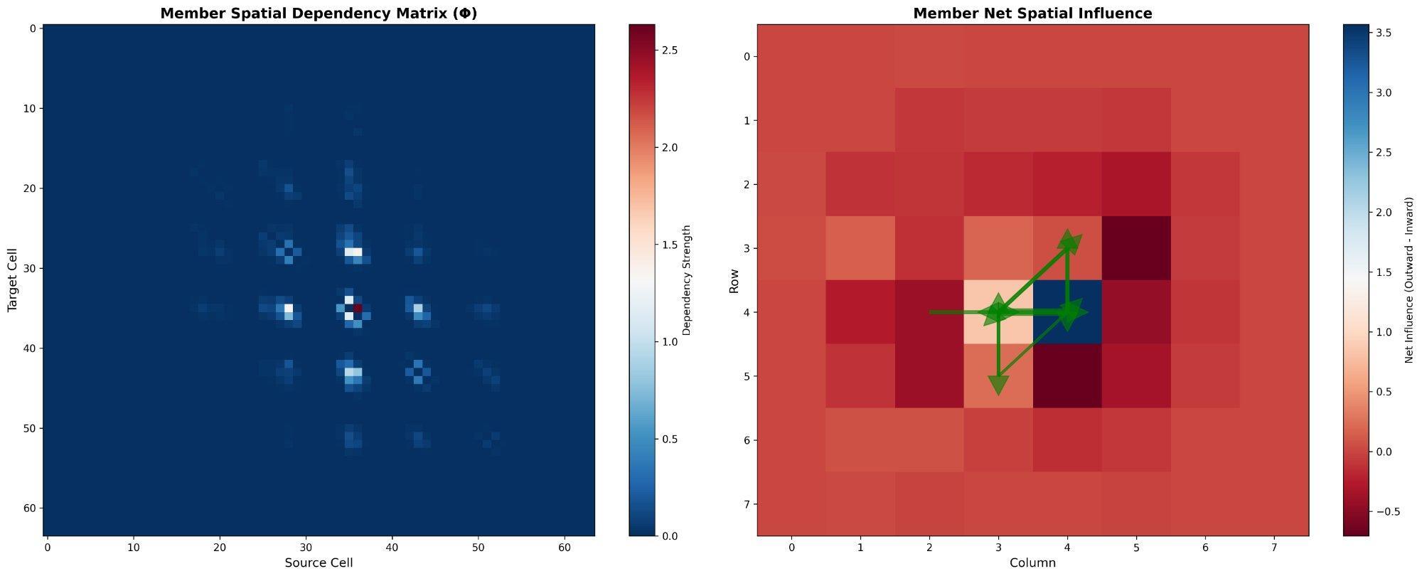
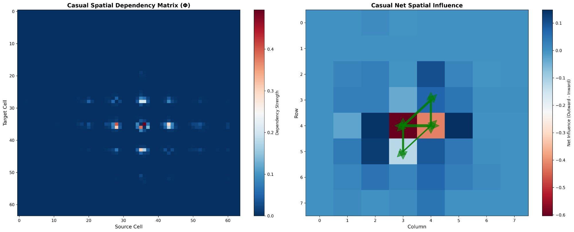
Spatial influence analysis. To quantify how demand history in one zone influences predictions in another, we applied a permutation test (Fisher et al. 2019). For each source zone, we removed its lagged demand signal and measured the resulting change in predicted demand across all target zones. Repeating this for all 4,032 ordered zone pairs produced a 64×64 influence matrix (Φ) for each user type. We summarized Φ using the anisotropy index, which quantifies the unevenness of influence distribution, and the proximity–influence correlation, which tests whether nearer zones exert stronger influence than distant ones. Full pseudocode appears in Supplemental Text S2.

3. Findings

We found that member demand is substantially more predictable than casual demand. The ConvLSTM explained 81.6% of variation in member pickups (R² = 0.816) versus 42.7% for casual pickups (R² = 0.427) (Table 1). Adding weather and temporal covariates improved predictions for both groups, but the gain was larger for casual users: R² increased by approximately 18% for casual demand versus 4% for member demand (Supplemental Tables S3–S4; Figure S4). Ridership exhibited a stronger positive correlation with temperature for casual users (r = 0.70) compared to members (r = 0.29). This divergence confirms that casual users possess a significantly higher weather sensitivity (Supplemental Figure S3).

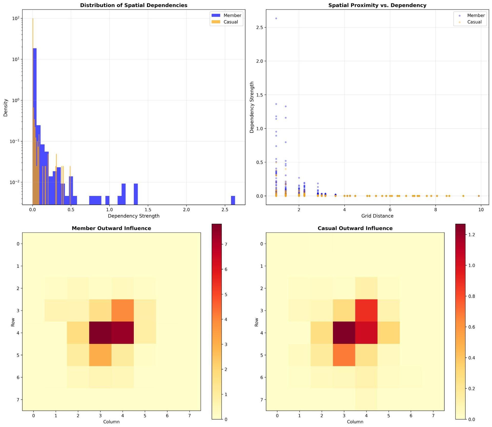
Q1. Proximity and spatial influence: Correlation analysis exhibited only a weak negative relationship between geographic distance and influence strength for both members (r = -0.164) and casual users (r = -0.131; Table 1). These weak negative values suggest that proximity does not determine how demand spreads across the network. Some adjacent zones showed little measurable connection during winter, while a small downtown cluster accounted for a disproportionate share of predictive signal. This pattern is consistent with evidence from New York City, suggesting that non-proximal spatial dependencies generalize across distinct urban contexts Miao et al. (2025).

Figure 2.Total pickups by grid zone for members (left) and casual users (right) across January 2026. Both groups concentrate in the same downtown cluster (zones 28–29, 36–37), but member totals are 4.5 times higher, consistent with the overall member–casual trip share

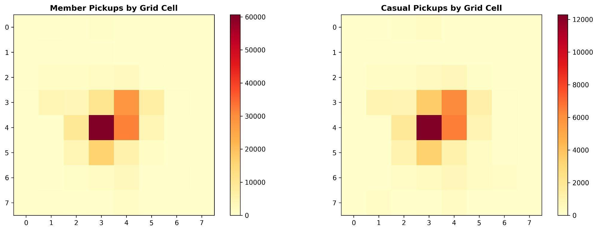
Q2. Member versus casual dependency structures: Members exhibited higher mean perturbation-based influence scores than casual users, with mean influence Φ roughly 5.5 times larger (Table 1). Because member trip volumes were also substantially higher, this difference should be interpreted as stronger model-estimated dependency in the observed demand field, not necessarily as a volume-normalized behavioral coupling. Although both groups concentrated pickups in the same downtown core (zones 28, 29, 36, and 37; Figure 2), influence mapping revealed structural differences invisible in raw demand totals. Most zones registered near-zero influence, but a small set of central cells acted as dominant predictive hubs (Figures 3–4). The anisotropy index exceeded 2.7 for members and 2.5 for casual users (Table 1), confirming that influence is highly concentrated rather than evenly shared. Notably, zones 36 and 37 contributed disproportionately to the predictive model, whereas most other zones played minor roles (Figure 5).

Q3. Weather data integration: Integrating weather variables and temporal covariates into the model, improved forecast accuracy for both groups, boosting members’ R² by 0.033 (+4.2%) and casual users’ R² by 0.066 (+18.3%). As members are regular commuters, the model improvement was more modest than for casual users (details are in Supplementary materials in Table S4 and Figure S4).

Figure 3.Member influence matrix (left): each cell shows how strongly the source zone (x-axis) shapes predicted demand at the target zone (y-axis). The matrix is sparse — most entries are near zero — with concentrated hotspots among downtown zones 28, 29, 36, and 37. Net influence map (right): red zones export more influence than they receive; blue zones are net receivers. Arrows show the strongest influence pairs.

Figure 4.Casual-user influence structure, showing substantially weaker overall dependence than the member matrix. The net influence map (right) suggests that casual demand is drawn toward the downtown core, but the pattern is weaker and less organized than for members.

Figure 5.Network-wide distribution of spatial influence for member (left) and casual (right) users. Red indicates zones with disproportionately high net influence; blue indicates net receivers. The concentration of member influence in the downtown core (zones 36 and 37) underscores the importance of these hubs for network-wide demand prediction.

From an operational perspective, the concentration of influence in zones 36 and 37 suggests these locations warrant priority in member-focused redistribution strategies. Because activity at these hubs predicts demand elsewhere, shortfalls there could propagate across the network. Our findings suggest that weather-responsive approaches such as pre-positioning bikes ahead of favorable conditions may be more effective for casual users than zone-to-zone redistribution. This acknowledges the high weather sensitivity and diffuse spatial footprint of casual riders. However, these are model-derived patterns, and require validation against operational data before specific planning decisions are taken.

Two limitations merit emphasis. First, Capital Bikeshare introduced a policy allowing riders to leave bikes outside full stations after our study period; our findings thus reflect pre-policy conditions and serve as a baseline for subsequent evaluation. Second, the 8×8 grid resolution, chosen for cross-study comparability, smooths over finer neighborhood-scale variation. Smaller zones could capture more local detail but would yield sparse winter data, particularly for casual riders. Grid sensitivity tests in Supplemental Table S2 show that the proximity–influence correlation remains weak and negative across all resolutions, confirming that the 8×8 grid is not a biased choice for this study. Finally, our results reflect winter-specific demand patterns in January 2026, DC’s coldest month; the spatial dependency structure may differ in other seasons when weather sensitivity and trip purposes shift.

Acknowledgements

The authors thank Capital Bikeshare (https://capitalbikeshare.com/system-data) for open trip data access and the Open-Meteo project (https://open-meteo.com/en/docs/historical-weather-api) free historical weather archives. During the preparation of this work, the authors used AI to improve readability and language style. After using this tool, the authors reviewed and edited the content as needed and take full responsibility for the publication.