Price Signals and Load Flexibility in Public Transport: A Cost Analysis of Electric Bus Charging

1. Questions

This study investigates how spatial and temporal flexibility in electric vehicle (EV) charging affects user costs under Sweden’s electricity tariff system. Most end-users pay separately for electric energy and grid connectivity. While consumers choose among energy providers, whose tariffs reflect wholesale market prices in Sweden’s four bidding areas (SE1–SE4), grid fees are charged by the local distribution system operator (DSO), which holds a natural monopoly over electricity distribution in one or more of the 311 non-overlapping network concession areas (as of 2024). Though set by the local DSO, network tariffs also capture costs from the national transmission system and regional distribution grids, where applicable. Wholesale energy prices are uniform within a bidding area but vary hourly (and may be settled over 15-minute increments, effective 30 September 2025); by contrast, most grid tariffs show relatively little time-of-use variation, while the 125 unique DSO tariffs in Sweden (as of 2024) provide significant spatial variation.

Electric vehicles can exploit both temporal and spatial tariff differences. To explore this potential, we analyze the charging costs of Skövde’s municipal bus fleet, assuming a transition from diesel to electric buses. Fleet charging is assumed to be cost-driven, constrained by route schedules. Building on prior grid-optimized load profiles (Najafi, Gao, Parishwad, Tsaousoglou, et al. 2025; Najafi, Gao, Parishwad, Pourakbari-Kasmaei, et al. 2025; Najafi, Gao, Wang, et al. 2025), we examine whether current tariffs incentivize such charging behavior.

We address three questions:

1. How do wholesale and local tariffs contribute to charging costs?

2. Do current price signals align with grid-optimal charging behavior?

3. Could revised grid tariffs strengthen incentives for spatio-temporal load flexibility?

The third question concerns whether improved tariff structures are possible, rather than the design of a tariff that achieves fully grid-optimal behavior, which would require assumptions about operations and scheduling beyond the scope of this study; we note this as a direction for future research.

2. Methods

The analysis focuses on variations in electricity costs across network concession areas operated by multiple DSOs in the Skövde municipal area (SE3 bidding zone, Västra Götaland). Hourly wholesale prices for 2024 were obtained from Vattenfall (2024); grid tariff data were sourced from the Swedish Energy Markets Inspectorate (2025).

For each DSO, annual grid cost $C^\mathrm{grid}$ is computed as: $$C^\mathrm{grid} = C^\mathrm{fixed} + C^\mathrm{power}\sum_m P_m + C^\mathrm{power,hl}\sum_{m\in\mathcal{H}^\mathrm{hl}} P^\mathrm{hl}_m + \sum_{h} C^\mathrm{energy}(h) E_{h} ,$$

$$\begin{aligned} C^{\mathrm{energy}}(h) = \begin{cases} C^\mathrm{energy, hl}, & \text{if } h\in\mathcal{H}^\mathrm{hl},\\[3pt] C^\mathrm{energy, ll}, & \text{if } h\notin\mathcal{H}^\mathrm{hl}. \end{cases} \end{aligned}$$ where:

• $C^\mathrm{fixed}$: Fixed charge, including regulatory charges and subscription fee (SEK),

• $C^\mathrm{power}$: Subscribed power capacity charge (SEK/kW),

• $P_m$: Subscribed power capacity (kW) in month $m$,

• $\mathcal{H}^\mathrm{hl}$: High load time period,

• $C^\mathrm{power,hl}$: High load power charge (SEK/kW),

• $P^\mathrm{hl}_{m}$: High load power (kW) during months $m$ in $\mathcal{H}^\mathrm{hl}$,

• $C^\mathrm{energy}(h)$: Energy transmission charge function (SEK/kWh) for hour $h$, where $C^\mathrm{energy, hl}$ is the charge for energy during high load period $\mathcal{H}^{\mathrm{HL}}$ and $C^\mathrm{energy, ll}$ is the charge for energy outside high load period.

• $E_{h}$: Energy (kWh) consumed in hour $h$.

These numbers are assumed to exclude VAT. High-load definitions vary by DSO (Table 1); tariff components are summarized in Table 2.

Hourly e-bus charging load profiles for the Skövde fleet are based on a representative day optimized to minimize local grid congestion (Najafi, Gao, Parishwad, Tsaousoglou, et al. 2025; Najafi, Gao, Parishwad, Pourakbari-Kasmaei, et al. 2025; Najafi, Gao, Wang, et al. 2025). Assuming static route schedules and charging behavior, the representative day is replicated across the year to approximate annual charging demand.

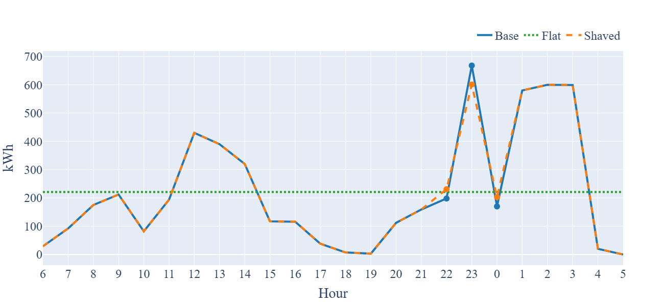
We consider three scenarios (Figure 1):

1. Baseline scenario: Uses the load profile from Najafi et al., which adjusts charging to optimize circuit-level distribution network operation without regard to end-use electricity costs. The pronounced drop at midnight occurs because buses are in transit returning to the depot during this hour, during which neither in-route nor depot charging is available.

2. Flat scenario: Redistributes total daily energy evenly across all hours, producing a flat load curve. This limiting case is illustrative of the minimal peak power load for a given energy consumption, although it is presumably operationally unrealistic.

3. Peak shaving scenario: Reduces the daily peak load from the base scenario by 10%, redistributing the shaved energy evenly to the two adjacent hours to maintain the same total energy consumption. This is presented as a more realistic, incrementally reduced-cost variant of the Baseline scenario. We use only the two adjacent hours to the peak to illustrate a minimal operational adjustment, as shifting load over longer periods (e.g., 4–6 hours) would require schedule changes beyond what is deemed as operationally feasible for the Skövde bus system.

Figure 1.The hourly load profile for the baseline, flat and peak shaving scenarios over the course of a representative day, starting at 06:00. The peak hour (23:00) and its two adjacent hours differs for the baseline and peak shaving scenarios; all other hours are identical in these cases.

3. Findings

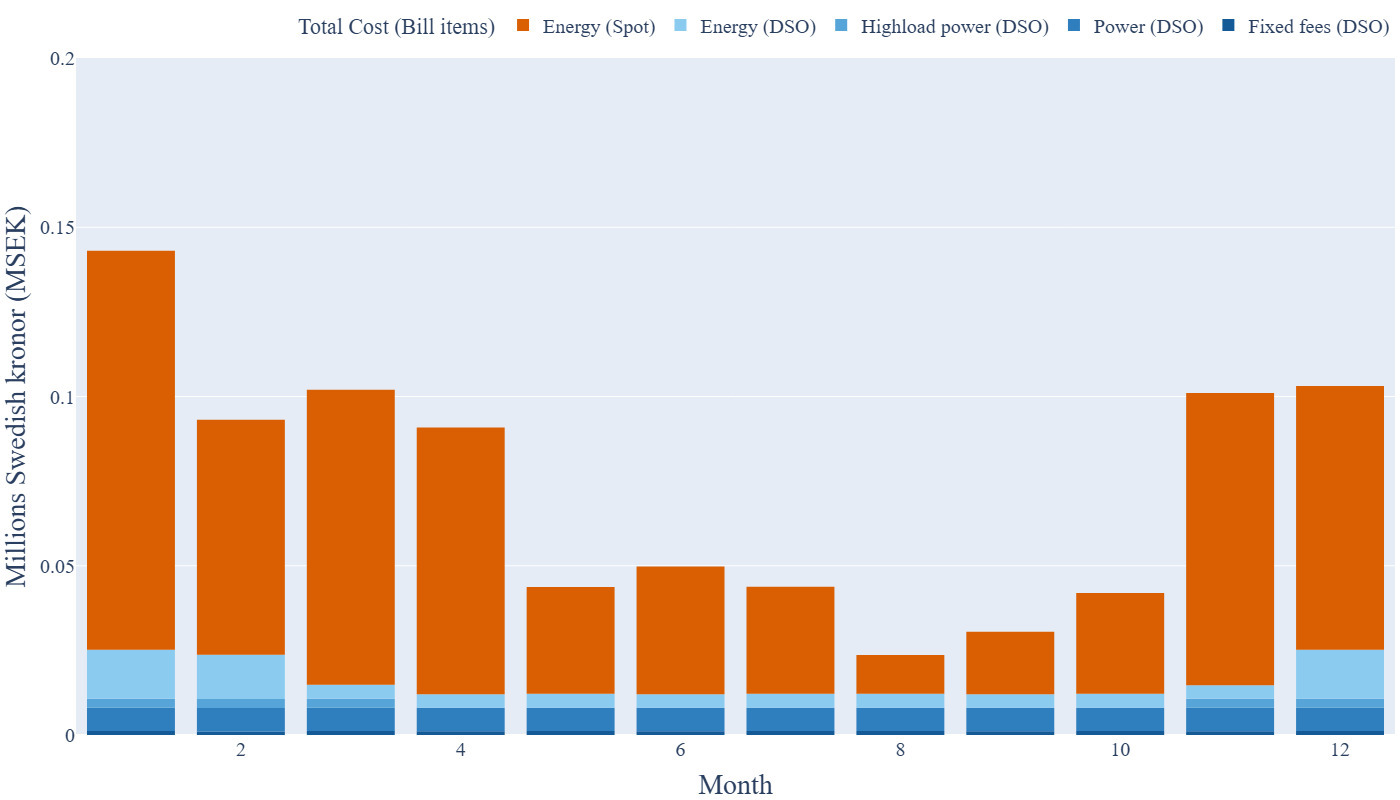
Figure 2 provides background on seasonal variation under Skövde Energi Elnät’s tariffs (2024). Wholesale prices show pronounced seasonality, driving large month-to-month differences in total cost, while network charges vary less across months. While this underscores that energy prices contribute substantially to total cost, public transport services with daily/weekly operating patterns cannot meaningfully shift charging across seasons; therefore, seasonal variation is informative context rather than a strategy for cost reduction in this application.

Figure 2.Monthly breakdown of total charging costs under Skövde Energi Elnät tariffs (2024). Fixed charges are distributed proportionally by month length (days). Wholesale prices drive pronounced seasonality; total monthly costs vary by a factor of 5 between the least- and most-expensive months.

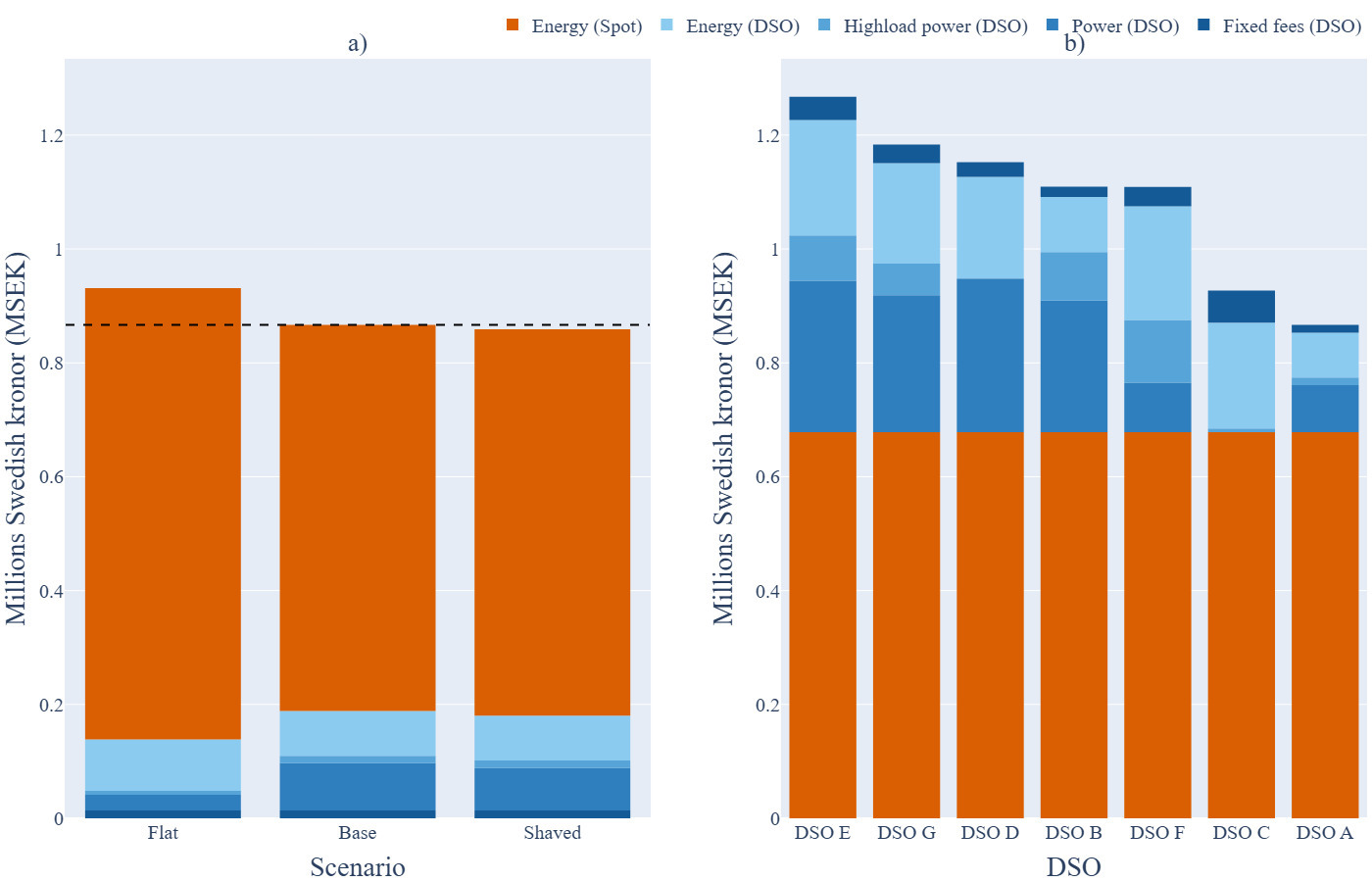
Figure 3a presents the implied end-use electricity costs of the three charging scenarios under Skövde Energi Elnät’s 2024 tariffs. The flat scenario has the highest total cost; while it eliminates demand peaks and minimizes subscribed power capacity charges, its evenly distributed profile shifts a substantial portion of charging to hours with higher wholesale prices. Because wholesale energy constitute the largest component of total cost, the Flat scenario performs poorly despite its low network-tariff charges.

Figure 3.(a) Scenario cost comparison for Skövde Energi Elnät tariffs (2024): the Flat scenario has the highest total cost due to increased consumption during high-price hours, while Peak-shaving achieves the lowest total cost via reduced subscribed power capacity charges. (b) Spatial cost comparison for the Baseline scenario across DSOs in the Skövde municipal area: Skövde Energi Elnät exhibits the lowest cost; Sjogerstads Elektriska Distributionsförening the highest (difference 46%). Differences reflect DSO-specific tariff structures; wholesale prices are uniform across SE3.

The Peak-shaving scenario lowers subscribed-capacity charges via a 10% peak reduction, while slightly increasing energy costs due to load redistribution. The net effect is a lower total cost than Baseline, showing that modest intra-day load adjustments can reduce costs without major operational changes (see also Table 3). The analysis does not identify the cost-minimizing profile, but Peak-shaving illustrates how tariff structures can create economic incentives for temporal load shifting.

Figure 3b compares Baseline costs across DSO concession areas within the Skövde municipal area. This illustrates the user cost implications of relocating the bus charging in Skövde (i.e., relocating the bus depot) to an adjacent service area. Despite common wholesale prices across these areas, total electrcity costs differ substantially among DSOs due to tariff structure differences. The lowest-cost DSO (Skövde Energi Elnät)is 46% below the highest-cost DSO (Sjogerstads Elektriska Distributionsförening). These differences illustrate the potential for spatial load shifting, if charging opportunities were available in neighboring concession areas even within a single municipal area. Wholesale energy costs could be minimized by temporal load shifting, but the effect would be identical in any of these network areas; by contrast, the tariff structures of different DSOs play a bigger role in encouraging spatial load shifting.

Overall, tariff design significantly affects charging costs and incentives for flexibility. Wholesale price variation dominates total costs and creates incentives for temporal load shifting, while network-tariff structures (particularly subscribed power capacity charges) influence the economic value of peak-shaving measures, and encourage spatial load-shifting, where possible. More targeted tariff designs could improve alignment between user economic incentives and distribution-grid conditions.

Acknowledgements

The research is supported by a research grant from JPI Urban Europe and The Swedish Energy Agency (e-MATS, P2023-00029).

ChatGPT was used to assist in formatting the text. The authors take full responsibility for all content.