Probabilistic Bike-Sharing Demand Forecasting under Changing Weather and Seasonal Regimes with Transformer-Based Models

1. Questions

Bike-sharing demand is often forecast with statistical or tree-based regression baselines that can achieve strong point accuracy but do not always provide well-calibrated uncertainty under regime changes. Transformer-based models and N-BEATS can fuse exogenous weather and calendar signals with seasonal regimes to learn nonlinear interactions that may improve robustness. We therefore ask: (RQ1) Under our forward-chaining temporal split that evaluates next-period generalization (UCI: 2011→2012; Seoul: Dec–May→Jul–Nov), how do TFT, Informer-lite, Transformer, and N-BEATS compare with RF/XGBoost for one-hour-ahead demand forecasting? (RQ2) Do 80% prediction intervals (P10–P90) remain calibrated during holidays/weekends and under extreme weather? (RQ3) Which calendar and weather covariates (including season/month and weather variables) are most influential according to TFT variable selection?

2. Methods

Datasets. We used the UCI Bike Sharing Dataset (hour.csv; Washington, DC) and the Seoul Bike Sharing Demand dataset (hourly). For UCI, the target is total rentals (cnt); we used the exogenous covariates season, holiday, workingday, weathersit, and the continuous weather variables temp, atemp, hum, and windspeed (excluding casual and registered). For Seoul, the target is Rented Bike Count; we retained only records with Functioning Day = “Yes” and used the available calendar covariates (Hour, Seasons, Holiday) and continuous weather variables (Temperature, Humidity, Wind speed, Visibility, Dew point temperature, Solar Radiation, Rainfall, and Snowfall). Table 1 summarizes sizes and time spans.

Forecasting task and splits. We performed one-hour-ahead forecasting with a fixed lookback window of 24 hours. To stress temporal generalization under changing seasonal and weather regimes, we used forward-chaining splits that evaluate next-period performance (i.e., next-period forecasting rather than a controlled seasonal-shift experiment): UCI train < 2011-11-01, validation 2011-11-01 to 2011-12-31, and test year 2012; Seoul train < 2018-06-01 (winter/spring), validation June 2018, and test July– November 2018 (summer/fall). All reported metrics are computed on the held-out test periods only.

Features. We used calendar and weather covariates available in each dataset. Categorical time variables (hour-of-day, weekday, month, season, and weather category where provided) were one-hot encoded. Continuous weather variables were standardized using training-set statistics; binary indicators (holiday, working day) remained 0/1. The target was transformed with log(1+y) to stabilize variance (Hyndman and Athanasopoulos 2021). For deep models, each training sample is a sequence of length 25: the past 24 observed demand values (standardized log-demand) with covariates, plus the target-time covariates with the demand value masked and an explicit observation flag.

Models. We compared: (i) Random Forest quantile regression using the empirical distribution over trees (Breiman 2001); (ii) XGBoost quantile models using the quantile loss objective (Chen and Guestrin 2016); (iii) N-BEATS (Oreshkin et al. 2020) with a three-quantile output head; (iv) a Transformer encoder baseline (Vaswani et al. 2017); (v) an Informer-lite encoder with temporal distilling for efficiency (Zhou et al. 2021); and (vi) a simplified Temporal Fusion Transformer (TFT) with variable selection, an LSTM encoder, and attention (Lim et al. 2021). All neural models were trained with the pinball loss for quantiles q∈{0.1,0.5,0.9} (Koenker and Bassett 1978). We did not implement a heterogeneous ensemble baseline (e.g., simple averaging across models) to keep the study focused on comparable single-model uncertainty; evaluating such ensembles remains future work.

Training protocol. Neural models used Adam (learning rate 1e-3), batch size 256, gradient clipping (1.0), and early stopping on validation pinball loss (patience 2, max 6 epochs for Transformer/Informer/TFT and max 8 for N-BEATS). RF used 200 trees (min_samples_leaf=2, max_features=0.7). XGBoost trained three separate models (one per quantile) with 200 estimators, max_depth=5, learning_rate=0.08, subsample=0.8, and colsample_bytree=0.8. We selected these hyperparameters by validation tuning: each model family was evaluated on the validation period and we report the configuration with the lowest validation pinball loss. All experiments used a fixed random seed (42).

Evaluation. Point accuracy was measured on the median (P50) using MAE, RMSE, and MAPE; we emphasize MAE because it is in bikes/hour and is directly interpretable for operations and capacity planning, while RMSE and MAPE are reported for completeness. Probabilistic quality used mean pinball loss and empirical 80% interval coverage and width (P10–P90). Because counts are nonnegative, negative predictions after inverse transform were clipped to 0. We also report stratified results for holidays and extreme weather to quantify shift robustness.

3. Findings

Overall accuracy and calibration. Table 2 reports test performance, where lower MAE/RMSE/MAPE indicates more accurate point forecasts, and P80 coverage closer to the nominal 80% indicates better calibrated uncertainty. On UCI, the lowest MAE is obtained by N-BEATS (51.33 bikes/hour) and XGBoost (51.79), followed by RF (52.70); the same ordering holds for RMSE and MAPE. TFT has higher MAE (55.90) but the best-calibrated intervals among neural models (P10–P90 coverage 72.14% vs 44.84% for N-BEATS and 46.14% for the Transformer), while XGBoost is sharp but under-covered (59.14% coverage with width 74.84). On Seoul, RF and N-BEATS achieve the lowest MAE (115.86 and 115.07), whereas Transformer-based encoders underperform (MAE ≥ 211.01) under this winter/spring→summer/fall split. In Seoul, train+validation contain 5,040 functioning-day hours drawn only from Winter/Spring, while the test period contains 3,425 hours drawn only from Summer/Autumn (mean temperature shifts from 5.24°C in train to 20.09°C in test). By contrast, UCI trains on a full year (2011) and tests on the next year (2012). Answering RQ1, tree models and N-BEATS provide the most accurate point forecasts across the two cities; answering RQ2, TFT yields the closest-to-nominal 80% coverage (81.11%) but with wider intervals (width 903.08), while RF is conservative (89.26% coverage).

Shift and regime analysis. Table 3 focuses on holidays and extreme weather, where “Normal” denotes non-holiday hours with no precipitation (UCI: weathersit≤2; Seoul: Rainfall=0 and Snowfall=0) and “Extreme weather” denotes precipitation regimes (UCI: weathersit≥3; Seoul: Rainfall>0 or Snowfall>0). In UCI, TFT coverage drops from 72.90% in normal conditions to 58.90% under extreme weather, indicating under-coverage when weather regimes are rare. XGBoost remains under-covered across all UCI regimes (58.60% normal, 62.10% holiday, 64.70% extreme). In Seoul, TFT is near nominal in normal conditions (81.80%), becomes conservative on holidays (95.80%), and under-covers during precipitation (68.00%). These results show that regime shifts primarily affect tail uncertainty even when MAE changes modestly (Gneiting and Raftery 2007).

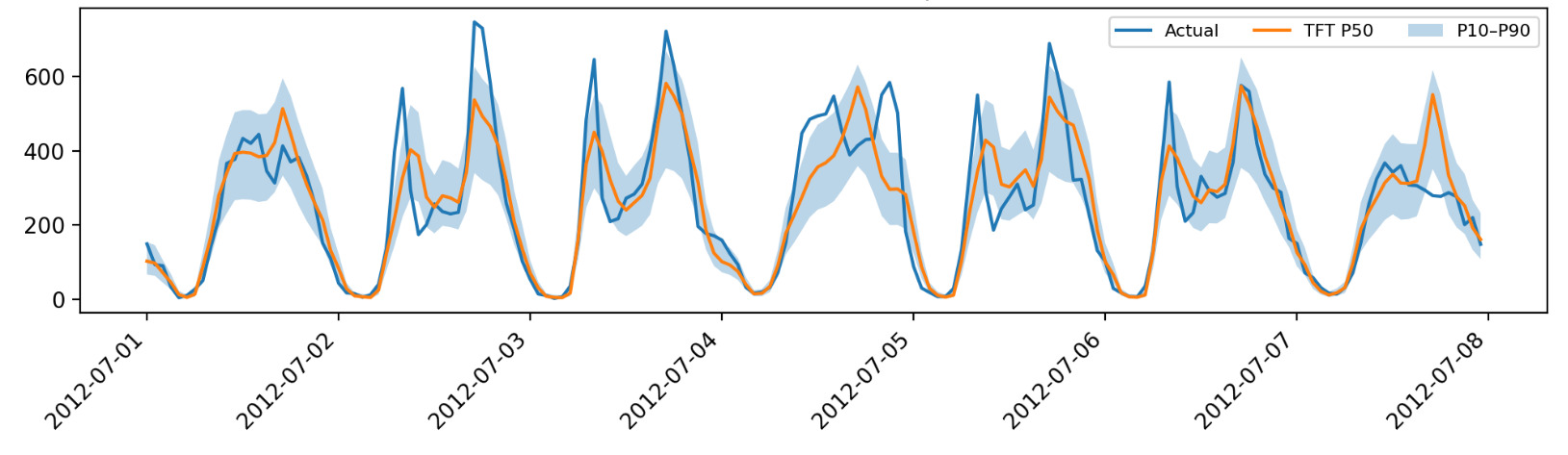
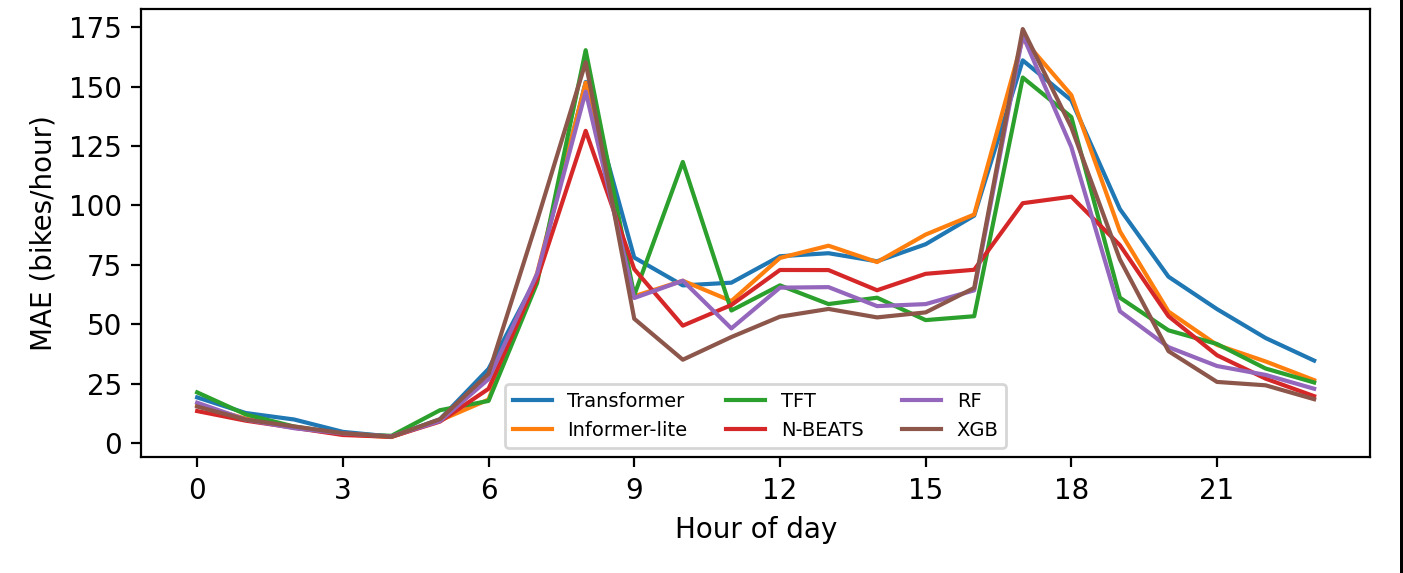
Case study and hourly structure. Figure 1 shows a holiday week in July 2012 where TFT’s interval expands around demand peaks and tightens during low-demand periods. Figure 2 decomposes MAE by hour-of-day in UCI: for every model, errors are higher at commuting (≈08:00) and evening (≈17–18:00) peaks than during overnight hours, reflecting heteroskedastic demand. N-BEATS exhibits the lowest MAE at most hours, suggesting it captures strong diurnal seasonality more effectively than the Transformer encoders in this one-hour-ahead setting.

Figure 1.UCI-DC: TFT probabilistic forecast (P10–P90), 2012-07-01–2012-07-07.

Figure 2.UCI: MAE by hour-of-day on the 2012 test set.

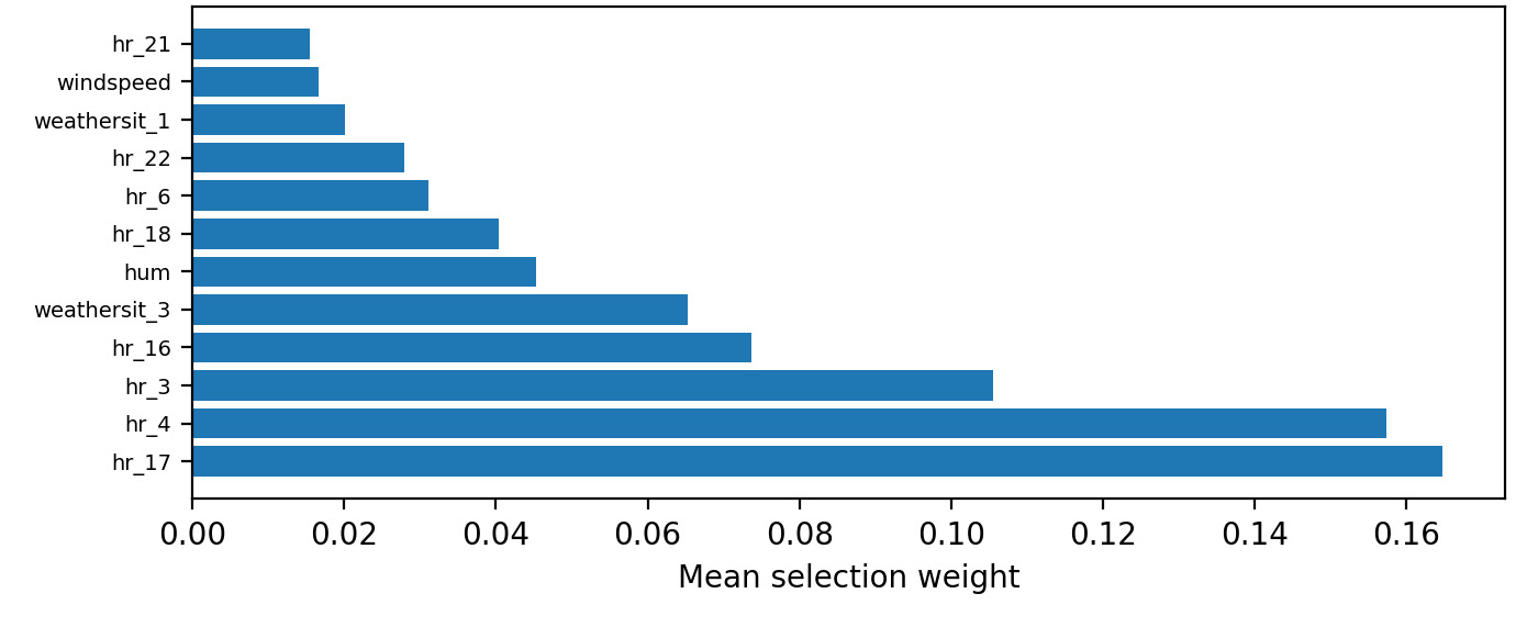
Interpretability. Figure 3 summarizes TFT variable selection weights. The most influential covariates include hour-of-day indicators (e.g., hr_17 denotes the 17:00 one-hot feature), seasonality indicators (month and season), and adverse weather categories (e.g., weathersit_3 denotes light rain/snow), along with continuous humidity (hum) and temperature variables (temp, atemp). For local explanation of the tree baselines, SHAP (SHapley Additive exPlanations) is directly applicable (Lundberg and Lee 2017), while TFT’s built-in selection provides a compact global ranking.

Figure 3.UCI: TFT variable selection weights (top 12 covariates).

Implications. Across two cities, strong point forecasts do not guarantee calibrated uncertainty: models with the lowest MAE often under-cover. For capacity planning and rebalancing, we recommend training with quantile losses and explicitly auditing coverage under holidays and extreme weather.

Code and Data Availability

https://github.com/bifoli/bike-demand-experiments

Acknowledgments

During the preparation of this work, the author(s) used ChatGPT in order to improve readability and language style. After using this tool, the author(s) reviewed and edited the content as needed and take(s) full responsibility for the content of the publication. All results, code, and citations have been rigorously verified by the authors for accuracy and integrity.