1. Questions
While qualitative descriptions of US streetcar history are plentiful (e.g. Warner (1978)) and there is a catalog of electric interurbans in the US (Hilton and Due 1964), no wide-scale quantitative studies of streetcars exist, with most being limited to singular cities or states (e.g. Xie and Levinson (2010)). This paper conducts a quantitative analysis of streetcar adoption, modelled under the framework of Rogers (1995) theory on the diffusion of innovations. S-curves for the adoption of technologies have often been studied, in fields ranging from electric vehicles (Graham 2022) to digital signal processors (Nieto, Lopéz, and Cruz 1998). We seek to answer the following questions:
-
What are the magnitudes and timing of streetcar system extents by metro area and state and the US national total, over 1894–1926? Where and when did the network peak?
-
Do these systems exhibit logistic S-curve growth, and does the growth rate vary systematically with timing?
2. Methods
We assemble annual series of in-service route-kilometres for streetcars and interurbans for selected metropolitan areas and for the United States total, drawing on the McGraw American Street Railway Investments directories and related sources listed in the Supplemental Information. Published between 1894 and 1932, these directories detail streetcar and electric interurban railway (hereafter collectively referred to as streetcar) systems by city, state and company. We use the length of track recorded in these directories to analyse the growth of streetcars in America.
Streetcar track lengths, as recorded in the McGraw Directories, are used to proxy for streetcar growth and adoption. We analysed the years between 1894 and 1926. The 1895, 1896, 1915 and 1916 directories were not available for analysis. Due to significant data discrepancies, 1912 and 1913 were not used for this analysis.
The original directories have been scanned and are archived by the HathiTrust Digital Library and are available online as PDFs. To turn them into a machine readable format, we processed the directories with ABBYY FineReader, an optical character recognition (OCR) program (ABBYY 2013).
Regular expression string matching was used to obtain a data table of track lengths by company, city, state and year. No distinction was made between local streetcar systems and interurbans, as often these would travel on the same tracks and were operated by the same organisation. Although the directories sometimes included incomplete track, or track under construction, only completed, operating track was kept. Mode (horse vs cable vs electric) was not kept.
The machine-extracted data was post-processed manually to increase accuracy. Validation was performed against hand-extracted values from 1894-1920 done previously as unpublished classwork by students at the University of Sydney.
For each series we model the cumulative route-kilometres \(S(t)\) as a logistic function of calendar year \(t\),
\[S(t) = \frac{K}{1+e^{-b(t-t_i)}} \tag{1}\]
where \(K\) is the long-run saturation level, \(b\) is the growth rate, and \(t_i\) is the inflection year, all variables defined in Table 1. We estimate the parameters \((K,b,t_i)\) for each city and for the national total by ordinary least squares on Equation (1), using all years with observed data. Modelling details are provided in the Supplemental Information. For each series we report the fitted parameters, the coefficient of determination \(R^2\), and the observed maximum route-kilometres and its year (Tables S1–S4).
The S-curve was only applied to the growth period, with the end of the growth period being determined by the year the maximum observed value occurred. S-curves were modelled by city and state, where the observed maximum was greater than 100 miles (160 km) of track, and more than five years of observed growth was available.
Table 1.Notation
| Symbol |
Meaning [units] |
| \(S(t)\) |
Track length at year \(t\) [km] |
| \(K\) |
Asymptotic maximum track length [km] |
| \(b\) |
Logistic growth rate parameter [1/year] |
| \(t\) |
Year [calendar year] |
| \(t_i\) |
Inflection year, where \(S=0.5K\) [calendar year] |
| \(T_{\max}\) |
Observed maximum track length [km] |
3. Findings
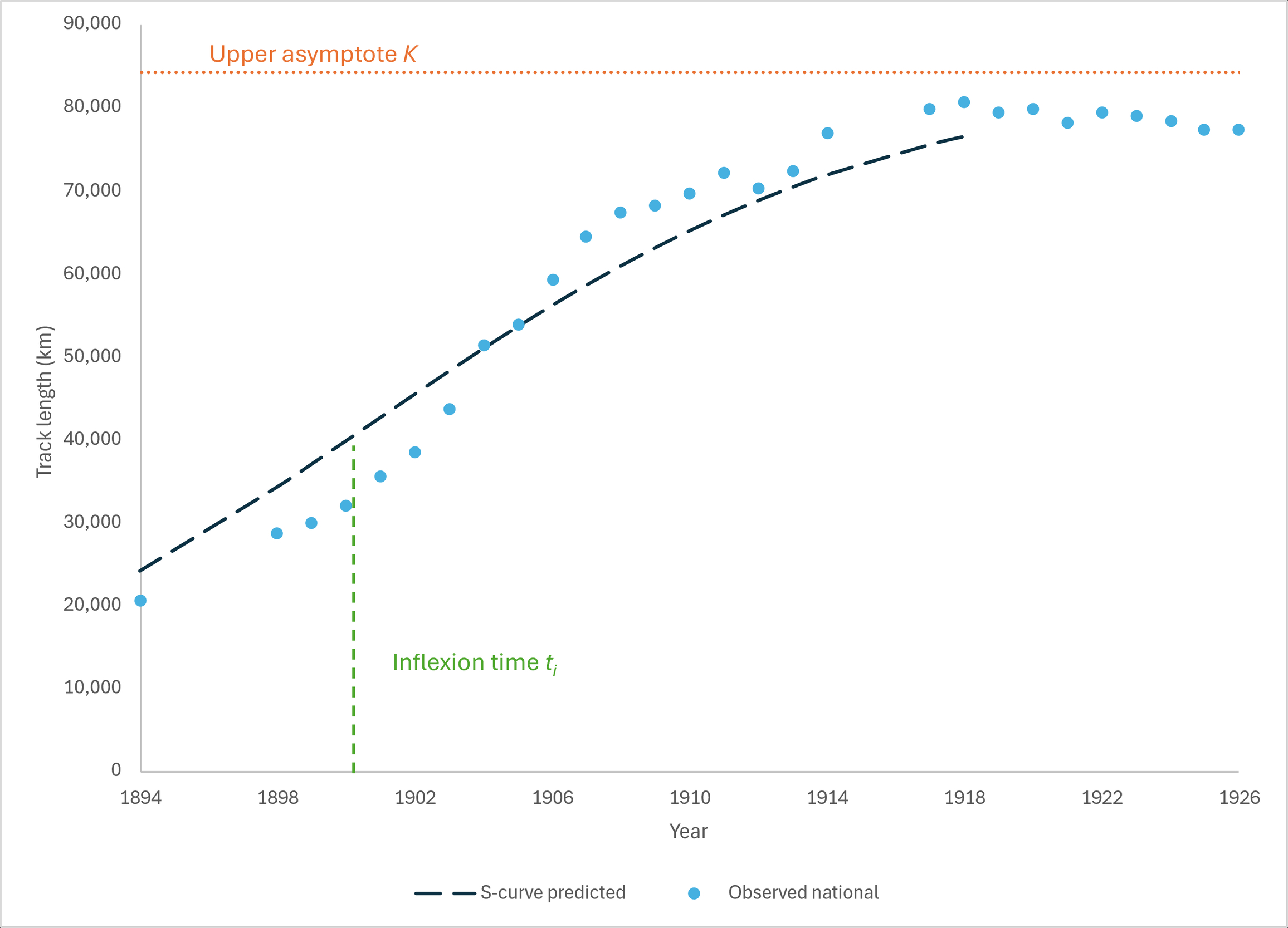
Figure 1.National United States S-curve. National total: United States observed maximum 80,660 km (1918); fitted \(K=84{,}208\) km; \(t_i=1901\); \(b=0.134\); \(R^2=0.89\)
3.1. Magnitudes and timing
We find that the United States reached an observed maximum of \(80{,}660\) km in 1918 (Figure 1).
The largest metro areas were Chicago, IL \(6{,}527\) km (1926), New York City, NY \(5{,}248\) km (1918), Boston, MA \(3{,}922\) km (1908), Los Angeles, CA \(2{,}388\) km (1920), Detroit, MI \(2{,}159\) km (1925), Pittsburgh, PA \(2{,}045\) km (1910). The median inflection year across metros is 1909. See Table 2 for details.
The most extensive streetcar systems were found in the following states: New York \(10{,}371\) km (1918), Illinois \(8{,}818\) km (1922), Pennsylvania \(8{,}468\) km (1914), Ohio \(7{,}011\) km (1907), California \(6{,}762\) km (1925), Massachusetts \(6{,}540\) km (1911). Across states, the median inflection year is 1903.5
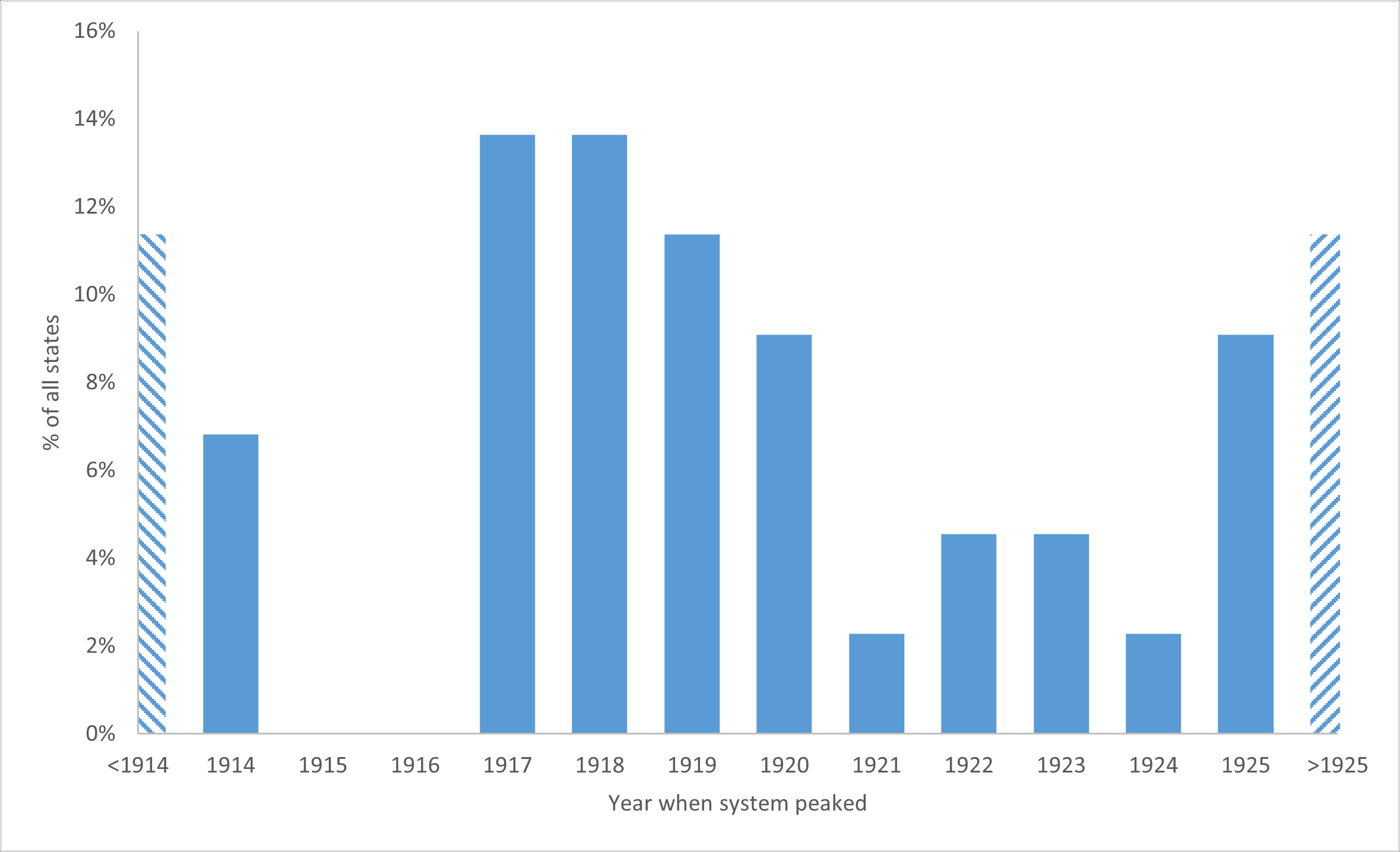
Only 14% of states peaked in the same year (1918) as the national system, most notably New York. The spread of peak years amongst states is varied across the 1910s and 1920s (Figure 2). 25 of 44 states peak by 1919, and 19 of 44 from 1920–1926. See Table 3 for details.

Figure 2.Proportion of states peaking by year
Table 3.S-curve statistics for states
| Location |
Obs. max. (km) |
Year obs. |
Theor. max. (km) |
\(b\)-value |
Inflection year |
\(R^2\) |
| Alabama | 673 | 1925 | 752 | 0.078 | 1902 | 0.9 |
| Arkansas | 211 | 1919 | 225 | 0.132 | 1901 | 0.83 |
| California | 6762 | 1925 | 6841 | 0.206 | 1907 | 0.92 |
| Colorado | 820 | 1910 | 898 | 0.175 | 1900 | 0.76 |
| Connecticut | 2598 | 1917 | 2676 | 0.194 | 1906 | 0.86 |
| D. C | 687 | 1918 | 766 | 0.121 | 1903 | 0.89 |
| Delaware | 256 | 1920 | 259 | 0.174 | 1905 | 0.58 |
| Florida | 327 | 1920 | 365 | 0.14 | 1907 | 0.97 |
| Georgia | 870 | 1924 | 948 | 0.098 | 1901 | 0.97 |
| Idaho | 190 | 1918 | 196 | 0.334 | 1910 | 0.87 |
| Illinois | 8818 | 1922 | 8896 | 0.156 | 1906 | 0.84 |
| Indiana | 4767 | 1908 | 4846 | 0.398 | 1903 | 0.75 |
| Iowa | 1739 | 1923 | 1819 | 0.145 | 1905 | 0.96 |
| Kansas | 889 | 1917 | 969 | 0.127 | 1911 | 0.65 |
| Kentucky | 842 | 1914 | 921 | 0.164 | 1904 | 0.8 |
| Louisiana | 528 | 1918 | 607 | 0.079 | 1899 | 0.84 |
| Maine | 930 | 1921 | 951 | 0.177 | 1902 | 0.95 |
| Maryland | 1147 | 1920 | 1226 | 0.135 | 1899 | 0.86 |
| Massachusetts | 6540 | 1911 | 6619 | 0.29 | 1898 | 0.91 |
| Michigan | 3548 | 1923 | 3627 | 0.138 | 1905 | 0.82 |
| Minnesota | 1363 | 1926 | 2021 | 0.068 | 1915 | 0.95 |
| Mississippi | 199 | 1918 | 214 | 0.205 | 1906 | 0.93 |
| Missouri | 1976 | 1914 | 2055 | 0.21 | 1898 | 0.9 |
| Montana | 449 | 1918 | 528 | 0.13 | 1913 | 0.72 |
| Nebraskaa | 369 | 1917 | 370 | 0.11 | 1889 | 0.29 |
| Nebraskab | 369 | 1917 | 398 | 0.123 | 1897 | 0.91 |
| New Hampshire | 487 | 1905 | 566 | 0.326 | 1901 | 0.8 |
| New Jersey | 2578 | 1920 | 2657 | 0.156 | 1900 | 0.91 |
| New York | 10371 | 1918 | 10449 | 0.224 | 1902 | 0.9 |
| North Carolina | 621 | 1922 | 700 | 0.153 | 1914 | 0.93 |
| Ohio | 7011 | 1907 | 7091 | 0.433 | 1900 | 0.81 |
| Oklahoma | 597 | 1926 | 616 | 0.252 | 1912 | 0.99 |
| Oregon | 1216 | 1925 | 1294 | 0.162 | 1909 | 0.94 |
| Pennsylvania | 8468 | 1914 | 8547 | 0.342 | 1900 | 0.93 |
| Rhode Island | 739 | 1917 | 740 | 0.271 | 1897 | 0.77 |
| South Carolina | 240 | 1919 | 278 | 0.112 | 1905 | 0.9 |
| Tennessee | 834 | 1926 | 1249 | 0.045 | 1913 | 0.88 |
| Texas | 1775 | 1919 | 1854 | 0.181 | 1906 | 0.81 |
| Utah | 822 | 1925 | 901 | 0.156 | 1911 | 0.92 |
| Vermont | 205 | 1917 | 209 | 0.177 | 1899 | 0.71 |
| Virginia | 777 | 1926 | 842 | 0.08 | 1894 | 0.61 |
| Washington | 1963 | 1919 | 2042 | 0.205 | 1906 | 0.94 |
| West Virginia | 1121 | 1919 | 1201 | 0.203 | 1909 | 0.95 |
| Wisconsin | 1303 | 1926 | 1329 | 0.138 | 1900 | 0.96 |
a When considering entire 1894-1926 period
b When considering post-1902 only
3.2. Trends
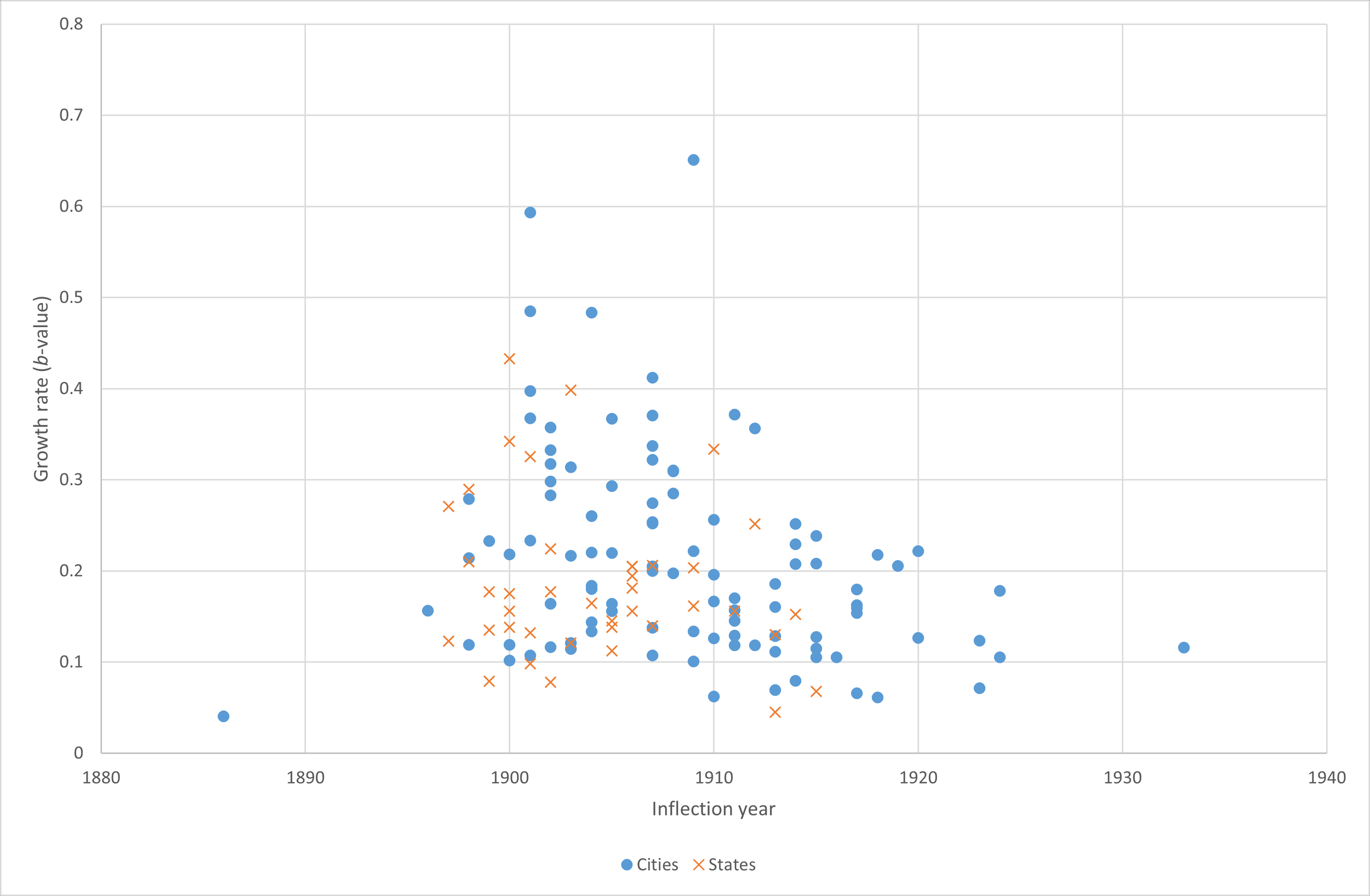
We do not find a robust increase in \(b\) for later \(t_i\) across metros or states (see Figure 3 and SI), indicating that institutional and financial factors likely dominate simple diffusion-timing expectations.
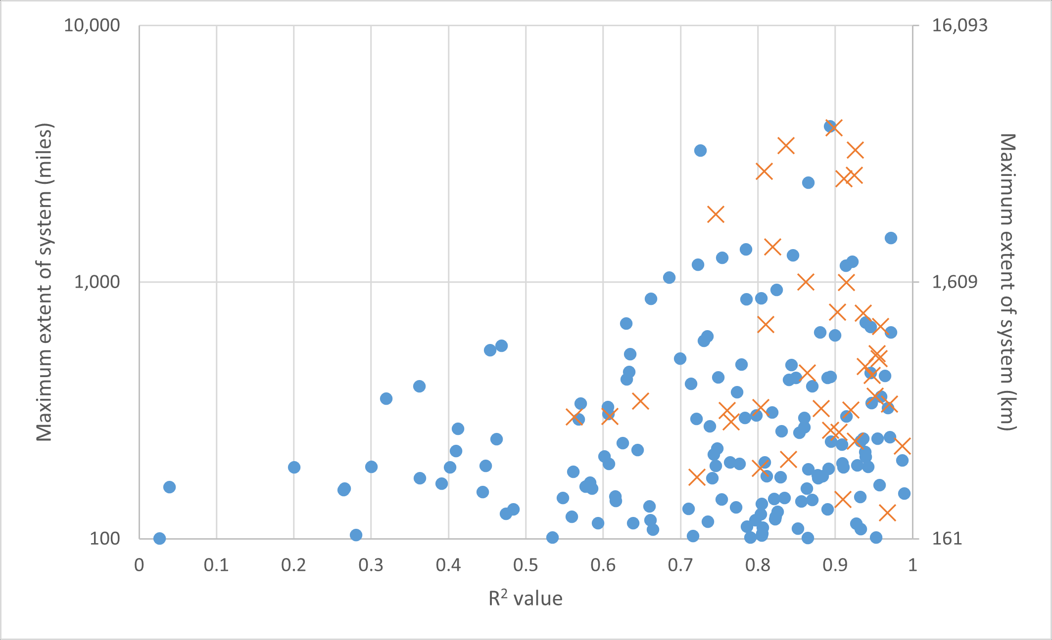
However, logistic fits are strong: 102 of 152 metros and 40 of 44 states have \(R^2>0.7\). We see that the aggregation to state-level improves the logistic fit, consistent with smoothing of local discontinuities (See Figure 4 and Figure 9; Table 2 and Table 3).

Figure 3.Estimated growth rate \(b\) versus inflection year \(t_i\).

Figure 4.\(R^2\) against maximum system length.
Table 2.S-curve statistics for cities with systems over 100 miles (160 km) at maximum extent
| Location |
Obs. max. (km) |
Year obs. |
Theor. max. (km) |
\(b\)-value |
Inflection year |
\(R^2\) |
| Akron, Ohio | 475 | 1926 | 499 | 0.133 | 1909 | 0.86 |
| Albany, New York | 280 | 1921 | 359 | 0.118 | 1911 | 0.83 |
| Allentown, Pennsylvania | 633 | 1924 | 711 | 0.105 | 1915 | 0.87 |
| Alliance, Ohio | 185 | 1905 | 264 | 0.341 | 1908 | 0.59 |
| Alton, Illinois | 220 | 1925 | 299 | 0.105 | 1924 | 0.81 |
| Altoona, Pennsylvania | 162 | 1910 | 241 | 0.205 | 1907 | 0.86 |
| Anaconda, Montana | 252 | 1917 | 332 | 0.1 | 1938 | 0.27 |
| Anderson, Indiana | 1075 | 1909 | 1154 | 0.483 | 1904 | 0.95 |
| Athol, Massachusetts | 235 | 1919 | 314 | 0.147 | 1925 | 0.62 |
| Atlanta, Georgia | 521 | 1923 | 600 | 0.107 | 1907 | 0.97 |
| Atlantic City, New Jersey | 343 | 1923 | 373 | 0.161 | 1913 | 0.74 |
| Auburn, New York | 185 | 1910 | 264 | 0.285 | 1908 | 0.93 |
| Aurora, Illinois | 354 | 1917 | 380 | 0.136 | 1915 | 0.41 |
| Baltimore, Maryland | 949 | 1914 | 1028 | 0.119 | 1900 | 0.73 |
| Birmingham, Alabama | 438 | 1926 | 605 | 0.066 | 1917 | 0.86 |
| Bloomington, Illinois | 293 | 1907 | 372 | 0.32 | 1908 | 0.56 |
| Bluefield, West Virginia | 256 | 1924 | 257 | 0.156 | 1909 | 0.04 |
| Boone, Iowa | 315 | 1920 | 394 | 0.222 | 1920 | 0.78 |
| Boston, Massachusetts | 3922 | 1908 | 4001 | 0.397 | 1901 | 0.86 |
| Bridgeport, Connecticut | 395 | 1914 | 406 | 0.298 | 1902 | 0.95 |
| Bridgeton, New Jersey | 310 | 1919 | 389 | 0.086 | 1927 | 0.45 |
| Brockton, Massachusetts | 770 | 1902 | 848 | 0.593 | 1901 | 0.78 |
| Buffalo, New York | 1027 | 1920 | 1106 | 0.116 | 1902 | 0.88 |
| Camden, New Jersey | 229 | 1905 | 307 | 0.164 | 1902 | 0.75 |
| Champaign, Illinois | 1380 | 1914 | 1460 | 0.371 | 1911 | 0.79 |
| Charlotte, North Carolina | 375 | 1922 | 454 | 0.205 | 1919 | 0.91 |
| Chattanooga, Tennessee | 161 | 1919 | 172 | 0.016 | 1833 | 0.03 |
| Chicago, Illinois | 6527 | 1926 | 9790 | 0.071 | 1923 | 0.89 |
| Chico, California | 350 | 1917 | 352 | 0.651 | 1909 | 0.94 |
| Cincinnati, Ohio | 1880 | 1908 | 1959 | 0.318 | 1902 | 0.72 |
| Cleveland, Ohio | 1394 | 1926 | 1421 | 0.119 | 1898 | 0.8 |
| Columbus, Ohio | 686 | 1906 | 764 | 0.333 | 1902 | 0.75 |
| Dallas, Texas | 672 | 1917 | 750 | 0.14 | 1914 | 0.63 |
| Danville, Illinois | 875 | 1908 | 954 | 0.396 | 1909 | 0.45 |
| Davenport, Iowa | 277 | 1923 | 356 | 0.079 | 1914 | 0.74 |
| Dayton, Ohio | 811 | 1905 | 890 | 0.429 | 1902 | 0.7 |
| Decatur, Illinois | 185 | 1911 | 264 | 0.185 | 1913 | 0.64 |
| Denver, Colorado | 525 | 1911 | 604 | 0.105 | 1900 | 0.61 |
| Des Moines, Iowa | 302 | 1926 | 312 | 0.156 | 1905 | 0.89 |
| Detroit, Michigan | 2159 | 1925 | 2237 | 0.138 | 1907 | 0.78 |
| Duluth, Minnesota | 277 | 1914 | 356 | 0.066 | 1913 | 0.36 |
| East Liverpool, Ohio | 163 | 1918 | 241 | 0.127 | 1920 | 0.79 |
| East St. Louis, Illinois | 542 | 1919 | 547 | 0.239 | 1909 | 0.57 |
| Easton, Pennsylvania | 216 | 1914 | 295 | 0.14 | 1910 | 0.66 |
| El Paso, Texas | 166 | 1920 | 229 | 0.159 | 1917 | 0.81 |
| Erie, Pennsylvania | 473 | 1925 | 546 | 0.105 | 1916 | 0.72 |
| Evansville, Indiana | 384 | 1918 | 455 | 0.196 | 1910 | 0.89 |
| Fairmont, West Virginia | 311 | 1921 | 389 | 0.208 | 1915 | 0.93 |
| Fort Dodge, Iowa | 282 | 1910 | 336 | 1.001 | 1909 | 0.81 |
| Fort Wayne, Indiana | 719 | 1907 | 798 | 0.396 | 1906 | 0.63 |
| Fort Worth, Texas | 305 | 1917 | 385 | 0.145 | 1911 | 0.91 |
| Fostoria, Ohio | 167 | 1925 | 167 | 0.251 | 1913 | 0.28 |
| Ft Wayne, Indiana | 494 | 1925 | 573 | 0.136 | 1915 | 0.61 |
| Galesburg, Illinois | 233 | 1904 | 311 | 0.295 | 1906 | 0.55 |
| Galveston, Texas | 249 | 1914 | 275 | 0.09 | 1916 | 0.26 |
| Georgetown, Massachusetts | 211 | 1906 | 290 | 0.412 | 1907 | 0.71 |
| Glens Falls, New York | 335 | 1919 | 414 | 0.207 | 1914 | 0.94 |
| Gloversville, New York | 205 | 1914 | 208 | 0.279 | 1898 | 0.83 |
| Grand Rapids, Michigan | 395 | 1908 | 473 | 0.314 | 1903 | 0.94 |
| Harrisburg, Illinois | 394 | 1926 | 591 | 0.301 | 1931 | 0.46 |
| Harrisburg, Pennsylvania | 306 | 1905 | 385 | 0.153 | 1905 | 0.4 |
| Hartford, Connecticut | 306 | 1919 | 307 | 0.149 | 1906 | 0.2 |
| Haverhill, Massachusetts | 337 | 1917 | 415 | 0.142 | 1915 | 0.6 |
| Hazleton, Pennsylvania | 201 | 1919 | 280 | 0.071 | 1924 | 0.47 |
| Highwood, Illinois | 307 | 1925 | 309 | 0.225 | 1912 | 0.3 |
| Houston, Texas | 226 | 1924 | 233 | 0.14 | 1911 | 0.62 |
| Indianapolis, Indiana | 1680 | 1908 | 1759 | 0.302 | 1905 | 0.69 |
| Jackson, Michigan | 671 | 1920 | 750 | 0.239 | 1915 | 0.84 |
| Jamestown, New York | 196 | 1914 | 275 | 0.17 | 1911 | 0.82 |
| Joliet, Illinois | 230 | 1906 | 309 | 0.293 | 1905 | 0.82 |
| Joplin, Missouri | 163 | 1914 | 241 | 0.222 | 1909 | 0.95 |
| Kalamazoo, Michigan | 244 | 1918 | 246 | 0.193 | 1907 | 0.44 |
| Kansas City, Missouri | 695 | 1924 | 768 | 0.114 | 1903 | 0.96 |
| Kittanning, Pennsylvania | 264 | 1920 | 343 | 0.102 | 1937 | 0.39 |
| La Salle, Illinois | 191 | 1909 | 269 | 0.242 | 1910 | 0.66 |
| Lancaster, Pennsylvania | 362 | 1908 | 441 | 0.22 | 1904 | 0.75 |
| Lansing, Michigan | 315 | 1907 | 394 | 0.304 | 1909 | 0.61 |
| Lawrence, Massachusetts | 258 | 1902 | 336 | 0.237 | 1901 | 0.58 |
| Lewiston, Maine | 316 | 1918 | 349 | 0.197 | 1908 | 0.91 |
| Lima, Ohio | 417 | 1917 | 422 | 0.371 | 1907 | 0.85 |
| Long Island City, New York | 1113 | 1911 | 1193 | 0.357 | 1907 | 0.63 |
| Los Angeles, California | 2388 | 1920 | 2467 | 0.254 | 1907 | 0.97 |
| Louisville, Kentucky | 500 | 1914 | 579 | 0.133 | 1904 | 0.82 |
| Memphis, Tennessee | 234 | 1926 | 253 | 0.102 | 1900 | 0.93 |
| Milford, Massachusetts | 176 | 1907 | 190 | 0.485 | 1901 | 0.93 |
| Milwaukee, Wisconsin | 712 | 1926 | 748 | 0.107 | 1901 | 0.95 |
| Minneapolis, Minnesota | 1025 | 1926 | 1392 | 0.069 | 1913 | 0.97 |
| Montreal, Quebec | 566 | 1922 | 566 | 0.134 | 1904 | 0.32 |
| Nashville, Tennessee | 284 | 1926 | 425 | 0.061 | 1918 | 0.88 |
| New Bedford, Massachusetts | 469 | 1920 | 549 | 0.1 | 1920 | 0.57 |
| New Haven, Connecticut | 1869 | 1926 | 2060 | 0.186 | 1913 | 0.91 |
| New Orleans, Louisiana | 386 | 1924 | 465 | 0.041 | 1886 | 0.93 |
| New York City, New York | 5248 | 1918 | 5327 | 0.18 | 1904 | 0.73 |
| Newark, New Jersey | 1504 | 1921 | 1539 | 0.184 | 1904 | 0.82 |
| Newton, Massachusetts | 210 | 1914 | 288 | 0.107 | 1911 | 0.48 |
| Norfolk, Virginia | 307 | 1910 | 386 | 0.26 | 1904 | 0.94 |
| Norristown, Pennsylvania | 266 | 1920 | 325 | 0.1 | 1914 | 0.58 |
| Norwich, Connecticut | 357 | 1918 | 436 | 0.145 | 1921 | 0.64 |
| Norwood, Massachusetts | 201 | 1923 | 209 | 0.251 | 1914 | 0.8 |
| Oakland, California | 601 | 1918 | 679 | 0.101 | 1909 | 0.77 |
| Ogden, Utah | 282 | 1923 | 360 | 0.218 | 1918 | 0.88 |
| Oil City, Pennsylvania | 192 | 1918 | 270 | 0.179 | 1917 | 0.82 |
| Oklahoma City, Oklahoma | 241 | 1919 | 259 | 0.356 | 1912 | 0.99 |
| Omaha, Nebraska | 232 | 1924 | 233 | 0.157 | 1896 | 0.83 |
| Oneida, New York | 190 | 1921 | 269 | 0.178 | 1924 | 0.8 |
| Oshkosh, Wisconsin | 163 | 1924 | 241 | 0.049 | 1933 | 0.53 |
| Peoria, Illinois | 1388 | 1920 | 1468 | 0.18 | 1916 | 0.66 |
| Philadelphia, Pennsylvania | 1932 | 1914 | 2010 | 0.218 | 1900 | 0.92 |
| Pittsburg, Kansas | 169 | 1921 | 171 | 0.309 | 1908 | 0.81 |
| Pittsburgh, Pennsylvania | 2045 | 1910 | 2124 | 0.283 | 1902 | 0.85 |
| Pittsfield, Massachusetts | 261 | 1917 | 274 | 0.31 | 1908 | 0.96 |
| Portland, Maine | 175 | 1917 | 175 | 0.236 | 1900 | 0.66 |
| Portland, Oregon | 1119 | 1925 | 1197 | 0.167 | 1910 | 0.94 |
| Providence, Rhode Island | 683 | 1918 | 690 | 0.233 | 1899 | 0.89 |
| Reading, Pennsylvania | 646 | 1922 | 726 | 0.115 | 1915 | 0.71 |
| Richmond, Virginia | 486 | 1917 | 565 | 0.126 | 1910 | 0.8 |
| Rochester, New York | 991 | 1914 | 1070 | 0.2 | 1907 | 0.73 |
| Rockford, Illinois | 380 | 1919 | 417 | 0.153 | 1912 | 0.63 |
| Sacramento, California | 431 | 1919 | 510 | 0.086 | 1930 | 0.41 |
| Salt Lake City, Utah | 544 | 1926 | 705 | 0.111 | 1913 | 0.95 |
| San Bernardino, California | 320 | 1922 | 340 | 0.229 | 1914 | 0.81 |
| San Diego, California | 476 | 1925 | 555 | 0.163 | 1917 | 0.78 |
| San Francisco, California | 1999 | 1925 | 2078 | 0.157 | 1911 | 0.75 |
| San Jose, California | 300 | 1919 | 378 | 0.128 | 1913 | 0.87 |
| San Luis Obispo, California | 165 | 1922 | 243 | 0.116 | 1933 | 0.72 |
| Saratoga Springs, New York | 179 | 1911 | 180 | 1.62 | 1909 | 0.79 |
| Schenectady, New York | 225 | 1917 | 227 | 0.367 | 1905 | 0.86 |
| Scranton, Pennsylvania | 401 | 1925 | 480 | 0.118 | 1912 | 0.97 |
| Seattle, Washington | 843 | 1914 | 922 | 0.151 | 1911 | 0.63 |
| South Bend, Indiana | 443 | 1907 | 521 | 0.337 | 1907 | 0.74 |
| Spokane, Washington | 681 | 1918 | 689 | 0.322 | 1907 | 0.85 |
| Springfield, Illinois | 423 | 1914 | 502 | 0.256 | 1910 | 0.83 |
| Springfield, Massachusetts | 326 | 1925 | 336 | 0.164 | 1905 | 0.99 |
| Springfield, Ohio | 912 | 1922 | 991 | 0.098 | 1930 | 0.47 |
| St. Louis, Missouri | 1001 | 1908 | 1080 | 0.214 | 1898 | 0.9 |
| Stockton, California | 178 | 1919 | 257 | 0.154 | 1917 | 0.81 |
| Syracuse, New York | 633 | 1917 | 686 | 0.098 | 1913 | 0.36 |
| Tacoma, Washington | 319 | 1910 | 341 | 0.233 | 1901 | 0.76 |
| Terre Haute, Indiana | 214 | 1924 | 237 | 0.129 | 1911 | 0.77 |
| Titusville, Pennsylvania | 188 | 1919 | 267 | 0.123 | 1923 | 0.74 |
| Toledo, Ohio | 765 | 1908 | 808 | 0.368 | 1901 | 0.84 |
| Trenton, New Jersey | 310 | 1921 | 315 | 0.219 | 1905 | 0.75 |
| Uniontown, Pennsylvania | 196 | 1908 | 275 | 0.239 | 1914 | 0.56 |
| Utica, New York | 209 | 1917 | 211 | 0.357 | 1902 | 0.89 |
| Washington, D. C | 687 | 1918 | 766 | 0.121 | 1903 | 0.89 |
| Waterloo, Iowa | 229 | 1917 | 240 | 0.252 | 1907 | 0.87 |
| Wheeling, West Virginia | 277 | 1917 | 290 | 0.217 | 1903 | 0.88 |
| Wichita, Kansas | 176 | 1924 | 220 | 0.128 | 1915 | 0.85 |
| Wilkes-Barre, Pennsylvania | 253 | 1921 | 332 | 0.062 | 1910 | 0.86 |
| Wilmington, Delaware | 252 | 1924 | 257 | 0.14 | 1908 | 0.59 |
| Worcester, Massachusetts | 483 | 1917 | 539 | 0.144 | 1904 | 0.91 |
| Youngstown, Ohio | 576 | 1914 | 650 | 0.274 | 1907 | 0.96 |
Submitted: December 10, 2025 AEST
Accepted: January 13, 2026 AEST