1. Questions
On January 20, 2025, the United States Department of Transportation (USDOT) issued an Order mandating that all DOT grants, loans, and contracts prioritize projects in communities with marriage and birth rates above the national average (“Order No. 2100.7” 2025). As of August 2025, no implementation guidance has been provided. The order raises concerns about alignment of transportation resources with demographics (Verlinghieri and Schwanen 2020) given the growing diversity of US households (Livingston 2018; US Census Bureau 2023), including more single-parent, multigenerational, and cohabiting families, many shaped by economic and structural barriers. Urban areas, which tend to have greater racial and economic diversity, often face different transportation disadvantages, while rural regions typically show lower average incomes. Tying infrastructure funding to marriage and birth rates risks reinforcing existing inequities (Karner et al. 2020). A demographic analysis comparing the proposed 2025 DOT policy with the Justice40 initiative similarly finds that such metrics shift funding away from lower-resourced and racially diverse populations and toward predominantly white areas (Barajas et al. 2025).
This study investigates the relationship between community-level marriage and birth rates and transportation burden to understand how mobility influences family formation. Longer commutes and higher travel costs can reduce the time and financial resources available for relationships, caregiving, and childbearing (Stutzer and Frey 2008). These dynamics reflect broader structural constraints in which transportation systems shape economic opportunity and household stability. Thus, we hypothesize that higher travel costs and longer commute times correlate with lower marriage and birth rates, as residents may delay or forgo family formation due to economic and time constraints. We assess whether USDOT’s funding priorities align with equitable transportation outcomes (see Karner et al. 2020) or inadvertently disadvantage underserved populations.
2. Methods
This analysis uses 2019–2023 American Community Survey (ACS) 5-Year data (US Census Bureau 2024) to explore how birth and marriage rates relate to transportation infrastructure and federal funding priorities. Table 1 describes the variables and preprocessing calculations. Although the National Center for Health Statistics provides birth data, county-level coverage is incomplete, so we used ACS data for its greater granularity. Birth rate was calculated using ACS table B13016 as the number of births in the last 12 months per 1,000 women aged 15-50 in the population. Marriage rate was calculated using ACS table B12001 and defined as the number of men and women reporting that they are married divided by the total population aged 15 and older, multiplied by 1000. Our approach follows prior demographic research that operationalizes marriage rate as the share of the population that is currently married (Barajas et al. 2025; Mather and Lavery 2010).
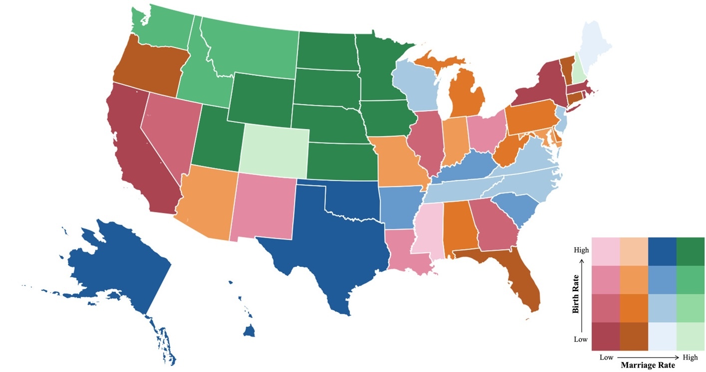
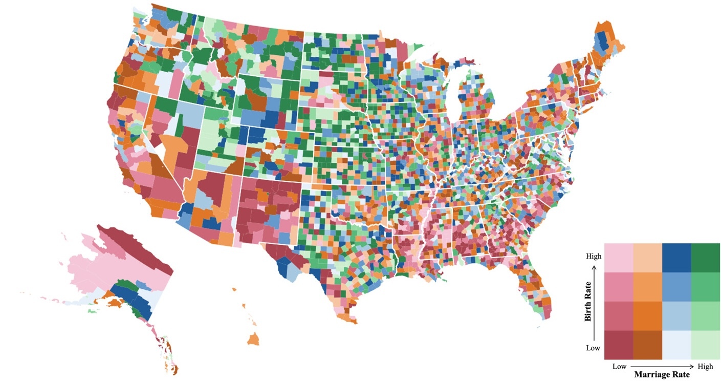
Data analysis was performed in R using the tidycensus package (Walker, Herman, and Eberwein 2025). Birth and marriage rates were first mapped across the US to identify spatial patterns. To construct the bivariate map, birth and marriage rates were each divided into quartiles. The lowest 25% of states were designated as low, the highest 25% as high, and the median represented the 50% threshold. Combining these quartile positions produced a 4×4 matrix of joint categories. State birth rates ranged from 28.24 to 65.15, with a median of 52.12. Marriage rates at the state level ranged from 328.90 to 562.98 and had a median of 505.02. At the county level, birth rates ranged from 0 to 443.04 and had a median of 54.24. County-level marriage rate had a range of 183.85 to 825.67, with a median of 523. 99.
We then conducted multivariate regression analyses at the state and county levels, modeling birth and marriage rates as dependent variables. Independent variables included demographics (poverty rate, median household income, education, race) and transportation factors (commute time, car access, homeownership rate). Variance inflation factor (VIF) checks identified multicollinearity between poverty rate and median household income at the state level (VIF > 10). Removing median household income reduced VIFs below 10 for all variables (Vittinghoff et al. 2012). ACS table B03002 was used for the race/ethnicity variables. Initially, the categories percent White (not Hispanic or Latino), Black (not Hispanic or Latino), Asian (not Hispanic or Latino), Hispanic or Latino of any race, and Other were used in the model. However, the inclusion of all categories introduced multicollinearity. After testing several alternative specifications, we found that using percent White (not Hispanic or Latino), Black (not Hispanic or Latino), Hispanic or Latino of any race, and Other provided a more stable and interpretable model. Percent Other is used as a reference category with all other races combined.
It is important to note that spatial dependence was considered, and we conducted Moran’s I tests to assess the extent of spatial autocorrelation in the dependent variables (birth rate and marriage rate) at the state and county levels. At the state level, birth rates had moderate clustering (Moran’s I = 0.38, p < 0.0001) and marriage rates showed weak and statistically insignificant clustering (Moran’s I = 0.10, p = 0.0817). At the county level, birth rates showed weak clustering (Moran’s I = 0.09, p < 0.0001), and marriage rates had mild clustering (Moran’s I = 0.28, p < 0.0001). These results indicate some degree of spatial autocorrelation, but it is not consistently strong across outcomes. Since spatial patterns were relatively weak overall and not significant for state-level marriage rates, a multivariate regression offers a justified and interpretable way to analyze these relationships. Nonetheless, future work could explore spatial models to further account for localized effects.
3. Findings
To examine birth and marriage rates across the US, we first mapped these rates at state and county levels (Figures 1 and 2). States with high marriage and birth rates are primarily in the Great Plains, Midwest, South Central, and Mountain West. Low marriage and birth rates cluster mainly in urbanized and coastal states. States with high marriage but low birth rates include several on the East Coast, Colorado, and Wisconsin, potentially reflecting older populations or delayed childbearing. States with low marriage and high birth rates are scattered, possibly indicating earlier family formation outside marriage.
.jpeg)

At the county level, patterns mirror those at the state level but with more local variation. Counties with low marriage and birth rates are widespread, while counties with high marriage and birth rates are mostly in the middle of the US and rural areas. Urban areas frequently show low birth and/or marriage rates, whereas rural regions tend to have higher rates. This spatial distribution suggests that allocating funding based on marriage and birth rates would shift resources toward rural populations. If county-level data guide distribution, the shift toward rural areas would be even more pronounced.
Multivariate regression at the state level (Table 2) found that longer commute times (p < 0.001), higher poverty (p = 0.0007), and higher education rates (p = 0.0009) predict lower birth rates. Percent White was also negatively associated with birth rates. Longer commutes may reduce time and energy for parenting, while poverty presents financial barriers to childbearing. Higher education, particularly among women, often delays family formation. Car access, homeownership, percent White, and percent Hispanic variables did not significantly predict birth rates at this level. The model explained 64% of the variation in state birth rates.
At the county level, higher birth rates were linked to shorter commutes (p < 0.001), higher car access (p = 0.0149), higher median household income (p = 0.0001), and lower education rates (p < 0.001). Percent White (p = 0.0247) and percent Hispanic (0.0079) were negatively associated with birth rates (Table 2). This combination suggests complex economic and cultural dynamics where economic disparity coexists with shorter commutes and lower education, influencing family size. Car access, homeownership, and percent Black were not significant, and the variance explained was low (adjusted R² = 0.07). This highlights the complex dynamics of modeling at the county level, where there are many other variables that affect birth rate.
For marriage rates (Table 3), higher poverty predicted lower marriage (p = 0.0006), reflecting economic insecurity’s impact on the decision or ability to marry. Higher car access predicted higher marriage rates (p = 0.0267), which shows that states where more households own vehicles tend to report higher proportions of married adults. Commute time and education were not significant predictors. The adjusted R² was 0.78.
County-level marriage rates were positively associated with car access (p < 0.001), homeownership (p < 0.001), and median household income (p < 0.001), and negatively with poverty (p < 0.001). Percent White and percent Hispanic were positively associated with marriage rates, while percent Black was negatively associated, reflecting broader structural inequalities. Factors such as incarceration rates, employment discrimination, and housing segregation likely contribute to lower marriage rates in counties with higher Black populations. Commute time was not significant. The model had a moderate fit (adjusted R² = 0.62).
Federal policy linking transportation funding to marriage and birth rates has substantial equity implications. Using them as funding criteria creates conflicting priorities, especially since these indicators are often negatively related, with high birth rates tending to coincide with low marriage rates, and both are associated with poverty. In practice, this approach would disproportionately benefit rural counties, which are whiter and less economically diverse, while disinvesting in urban areas where poverty, low marriage rates, and higher birth rates converge alongside acute transportation needs. This risks deepening inequities while expanding investment in rural and car-dependent infrastructure with limited public transit options (Hemmersbaugh, 2025).