1. Questions
Most trip distribution models allocate flows across all origin–destination pairs using a global rule (e.g., gravity/entropy (Erlander and Stewart 1990; Wilson 1970) or discrete choice (Domencich and McFadden 1975; Ben-Akiva and Lerman 1985)), or via sequential acceptance without explicit destination capacity (Intervening Opportunities (Stouffer 1940), or Radiation (Simini et al. 2012)), or using hiring dynamics (Tilahun and Levinson 2013). These approaches usually treat the network implicitly. A broad comparison with gravity/entropy, discrete choice, intervening opportunities, radiation, and ABODE appears in Table 1.
In contrast, we examine a cost-ordered, percolation-like expansion that depletes destination capacity as it is reached. With shortest-path costs the global benchmark is the Hitchcock–Koopmans transport problem (a min-cost flow on the OD bipartite graph) (Hitchcock 1941; Koopmans 1949; Dantzig 1951; Burkard, Klinz, and Rudolf 1996).
Our main question is:
- Can we construct an origin–destination matrix that respects destination opportunity constraints using only shortest-path costs and a fixed, reproducible order, without estimating behaviour?
Under what conditions is this approach like or unlike existing approaches? For instance, under a one-parameter acceptance rule with scaling factor, do expected flows reduce to a singly-constrained exponential-gravity form when no destination reaches its capacity? Similarly, under what cost/topology conditions does the greedy, cost-ordered allocation coincide with, or diverge from, a min-cost-flow solution?
2. Methods
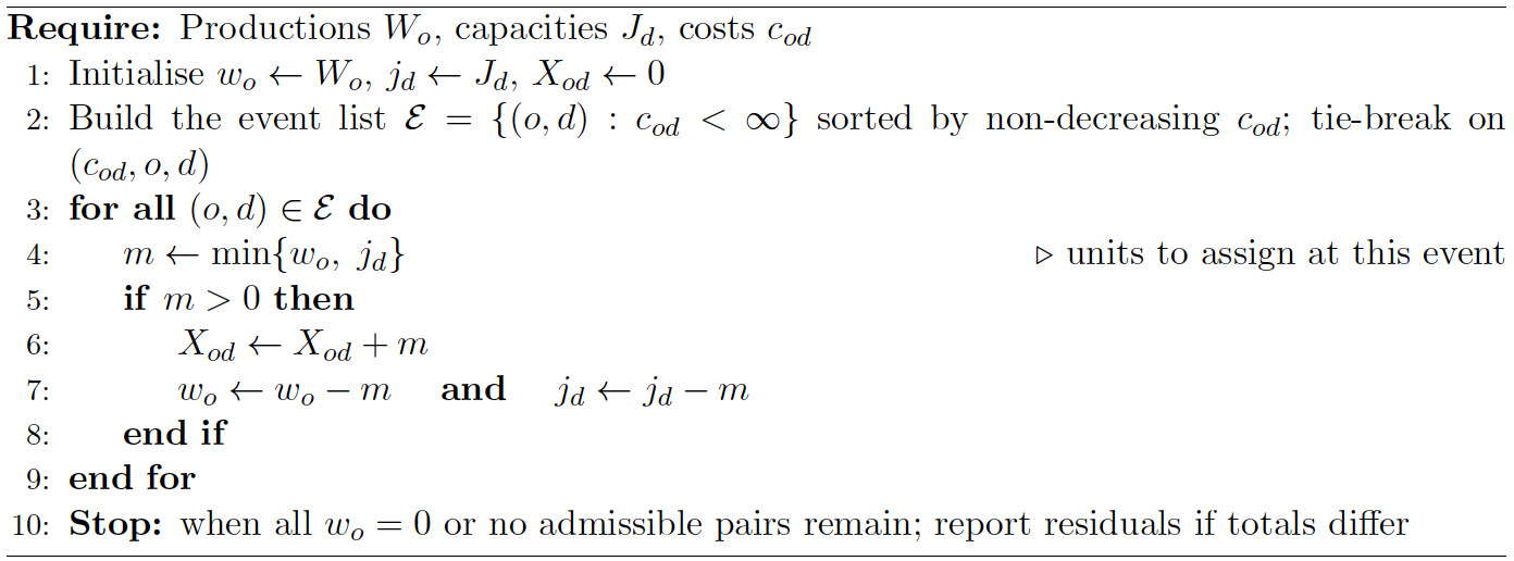
The Network Origin–Destination Estimation (NODE) method allocates workers from origins to jobs at destinations by sweeping feasible origin–destination pairs in non-decreasing (weakly increasing) shortest-path cost assigning until either the origin’s residual production or the destination’s residual capacity is exhausted.
Objects and data types. Let and where if is unreachable from on network Residuals are and Ties in are broken by a fixed lexicographic order on for reproducibility. Destination capacity is explicit and enforced at assignment time; link capacities are not modelled here and are handled in a subsequent route-choice/assignment step coupled to NODE.
NODE works as a percolation-like sweep over the network: as lower-cost states ‘open,’ new pairs become admissible; assignments proceed in cost order until destination capacities ‘close’ further flow. Admissible means (reachable over
NODE assumes:
-
A set of origins with productions (resident workers)
-
A set of destinations with attractions (jobs)
-
A transport network that yields generalised costs between and
The method applies a best-first expansion over the network. Any cost-ordered search algorithm (e.g., Dijkstra) can be used; what matters is the order in which destination candidates are discovered by increasing Ties are broken lexicographically for reproducibility. Equal-cost ties can be shared or randomised if desired. A deterministic choice can bias split patterns when ties are common, such as grid networks. NODE constructs a single OD matrix from zonal totals and shortest-path costs. This is shown in Algorithm 1.
.png)
It is not inherently a dynamic propagation model like the cell transmission model (CTM) (Daganzo 1994, 1995) or cellular automata (Nagel and Schreckenberg 1992), which evolve link states in time, though it could be used in such an evolutionary way. It can also be used in feedback with an agent-based route choice (ARC) model by supplying capacity- and topology-aware OD seeds (Zhu and Levinson 2018).
Acceptance and hazard. Let be the CDF and the PDF. With hazard the standard relation is
\[\small{f(c)=\lambda(c)\exp\!\Big(-\int_{0}^{c}\lambda(s)\,ds\Big), \quad F(c)=1-\exp\!\Big(-\int_{0}^{c}\lambda(s)\,ds\Big).}\tag{1}\]
With constant and if no destination reaches its capacity and acceptance draws are i.i.d. across the expected NODE flows reduce to the origin-constrained exponential gravity form:
\[\mathbb{E}[X_{od}] \;=\; W_o\frac{J_d e^{-\lambda c_{od}}}{\sum_{d'\in D}J_{d'}e^{-\lambda c_{od'}}}.\tag{2}\]
Here has units of if is time; in a discrete-time realisation with step the per-step acceptance is
Relation to social networks. The acceptance hazard can incorporate social pull. Prior work shows that social ties systematically shape activity locations and distances, strong ties meet closer or in-home, weak ties meet farther, while contacts mediate information about homes and jobs, influencing where people live and work (Tilahun and Levinson 2011, 2013). In NODE, we can encode this by adjusting the impedance or acceptance rate to account for the strength or share of an origin’s contacts near the destination.
CTM realisation (summary; full details in SI). NODE can be implemented over a time-expanded network. We partition space into cells (states); is a row-stochastic movement kernel of size giving the probability that mass moves between cells per at step The per-step acceptance applies to arrivals at destination cell (we allow to depend on in the SI). Algorithm 2 in the SI defines the state updates explicitly and shows how destination capacity is enforced before splitting across origins.
Incremental and evolutionary application. When a prior trip table exists and jobs or workers change, one can run NODE on residual changes (deltas), or apply a damped rolling reallocation; this yields incremental, not equilibrium, updates, consistent with evolutionary planning ideas (Levinson 1995), aligned with short-run rather than long-run changes.
NODE can also be implemented in an evolutionary frame across scenarios or time steps, in this case consider as costs and capacities change, Compare allocations via and record the costs at which destinations fill (frontier ‘closure costs’). The frontier closure cost of destination is the maximum cost at which any assignment to occurs in the sweep. This reveals who gains or loses under proposed links, prices, or shocks, and where capacity competition binds.
Position in the literature. NODE differs from gravity/entropy and discrete choice by allocating in cost order with explicit destination capacity and no global utility or balancing multipliers; it differs from intervening-opportunities and radiation by using network shortest-path costs rather than rank by distance or opportunities, and by enforcing capacity at assignment. It coincides in expectation with origin-constrained exponential gravity under the non-binding, single-hazard case above, but it generally diverges when capacities bind, topology reorders the reachable set, or hazards vary across places or groups.
3. Findings
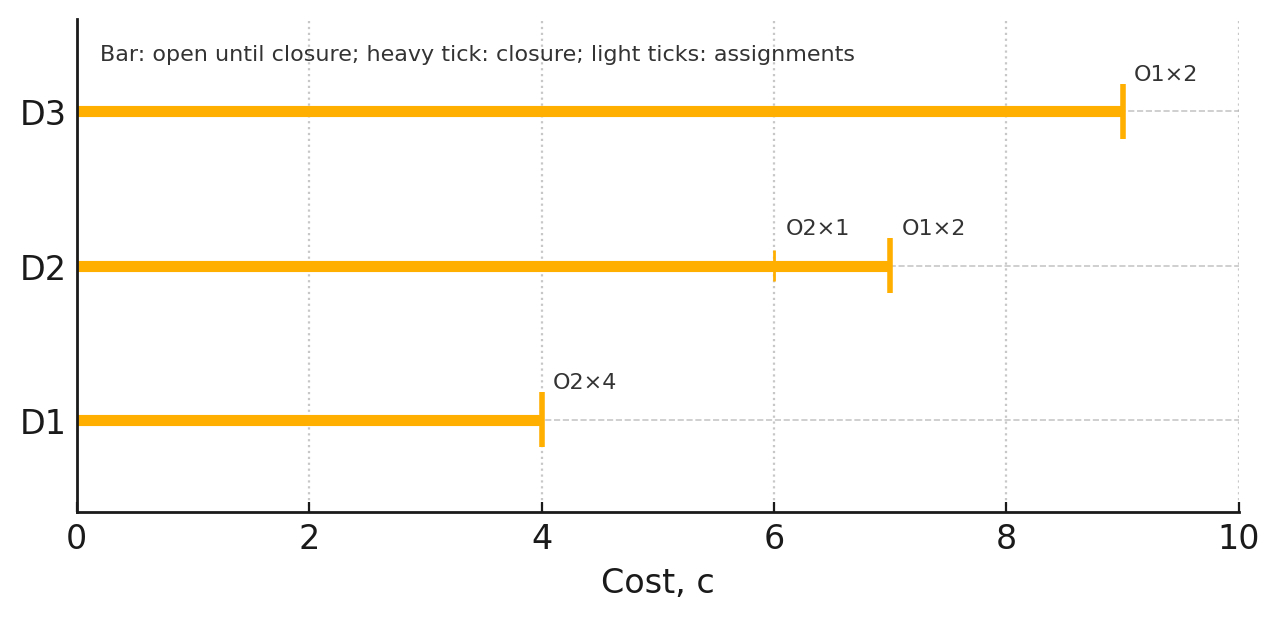
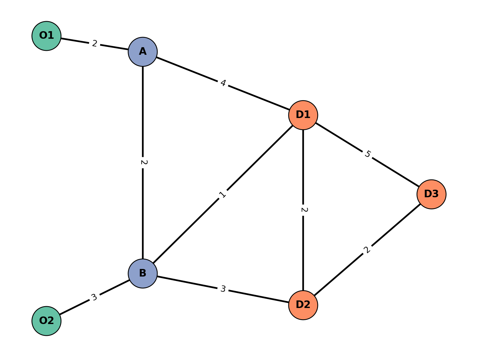
Worked example. Consider two origins with resident workers and and three destinations with job capacities Link costs determine on a small network (Figure 2).

_for_realised_allocations.jpg)
The first sweep fills from which reaches it earlier in cost order; then sends one worker to Unable to access sends two workers to and its remaining two to The realised allocation (Table 2) matches production and attraction totals, and shows diversion caused by competition. For stepwise clarity, residuals are updated as and assignments as
Stochastic draw. Table 2 also reports a single Monte Carlo realisation with i.i.d. acceptance. Row and column totals match and by construction, but the split across destinations differs from the deterministic sweep because some earlier candidates are declined.
Equivalence to gravity. With a single in and negligible destination capacity constraints, the expected NODE flows converge to those from a singly-constrained gravity or entropy-maximising model with the same impedance curve. This holds with a single hazard i.i.d. acceptance independent across destinations, connected OD pairs, and capacities that are never reached. In this limit, NODE is simply a different solution process that preserves the same trip length distribution.
Relation to min-cost flow (summary; SI has details). The deterministic sweep is not a general solver for the Hitchcock–Koopmans transport problem. However, when the OD cost matrix satisfies the Monge property a greedy order consistent with non-decreasing yields an optimal transport plan; see SI (Proposition A.1) and (Burkard, Klinz, and Rudolf 1996). Outside these conditions, NODE can diverge from the min-cost solution, which we illustrate with a counterexample in the SI.
Departures from gravity. Systematic differences arise from:
-
Capacity competition: Destinations reached early can fill, diverting later arrivals to further alternatives.
-
Topology effects: Network structure and asymmetries reorder which destinations are encountered first; cost ties (destinations reached at equal cost) and branching can produce distinctive spatial patterns.
-
Heterogeneity and stochasticity: Varying across groups or places, or random acceptance, breaks proportional balancing while preserving production and attraction totals.
When no destination reaches its capacity and costs produce a unique non-tied order, the deterministic sweep matches any allocation consistent with that order, though it need not be globally min-cost when later ties or alternative paths exist.
Implications. NODE is a transparent, network-based allocation method that exactly preserves zonal totals when totals match and pairs are connected, embeds topology and capacity directly in the search process, and can reproduce plausible trip length distributions without explicit global calibration. It is well-suited to:
-
Seeding OD matrices when only productions, attractions, and a network are known.
-
Capacity-limited facility allocation problems.
-
Benchmarking or coupling with route choice schemes that update costs between batches.
Even without behavioural detail, NODE is useful when capacity, topology, or sparse data make conventional gravity or utility-based models less appropriate.