Access Surplus: Valuing Accessibility by Integrating Opportunity Supply and Willingness to Pay

1. Questions

Most accessibility indices either count opportunities within a generalised cost cut-off, or weight them by an impedance function. They are simple, yet cut-offs are arbitrary, and fixed weights are hard to defend (Hansen 1959; Weibull 1976; Geurs and Wee 2004; Wu and Levinson 2020).

Utility-based indicators grounded in discrete choice use the logsum as an accessibility measure and derive consumer surplus for appraisal (Geurs, Wee, and Rietveld 2013; Niemeier 1997; Handy and Niemeier 1997). Logsum measures are welfare-consistent, but they rely on a utility specification, a defined choice set, and a common scale across models (Williams 1977; Small and Rosen 1981; Train 2009). Practice also uses the ‘rule of half,’ which can be read as an accessibility interpretation of user benefits as an alternative to Logsum measures (Fosgerau and Pilegaard 2021). Recent work improves cumulative opportunity metrics by introducing diminishing returns to additional nearby opportunities, addressing over-counting when each extra destination is weighted equally (Roper, Ng, and Pettit 2023). What remains missing is a welfare index that operates on the ranked opportunity set, keeps option value and generalised cost as separate objects with common units, aggregates cleanly across people, and can align with, yet not depend on, a particular choice model. This paper fills that gap by defining a surplus of access while avoiding arbitrary distance cut-offs.

We ask whether a measure can value the marginal option in generalised cost units (time or money, including private or social costs (Cui and Levinson 2018)), avoid cut-offs, aggregate cleanly across residents, and remain transparent. We introduce access surplus (\(\mathbb{A}\)) as the net area between a decreasing willingness-to-pay-by-rank curve, \(D_i(q)\), and the dual cumulative opportunity cost curve, \(S_i(q)\).

2. Methods

Primal (Hansen) cumulative opportunities. Perhaps the most common access measure is cumulative opportunities (Hansen 1959):

\[ A_i(t) = \sum_j O_j\, f_t(c_{ij}), \qquad f_t(c)= \begin{cases} 1 & c \le t,\\ 0 & c > t. \end{cases}\tag{1} \]

\(A_i(t)\) is the number of opportunities reachable within \(t\). Let \(c_{ij}\) be generalised cost from origin \(i\) to destination \(j\), and let \(O_j\) be the size of the opportunity at \(j\).

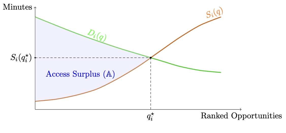
Dual access. Primal counts “how many by time.” But people often think in “how long until I can reach some number of places?” terms. Dual Access (Cui and Levinson 2020) captures that inverse idea by reading generalised cost (most typically travel time) off the sorted travel costs. Thus it is the cost of reaching a marginal additional opportunity. Concretely, the supply curve is just the \(q\)-th order statistic:

\[ S_i(q) = c_{i(q)} \quad \text{for } q=1,2,\dots,J_i .\tag{2} \]

This profile is typically S-shaped in cities: quick gains nearby as area (and thus, typically, opportunities) increases with the square of distance or travel time, then slower gains as one nears the edge where the set of distinct places levels off and density drops. This is illustrated in Figure 1.

Demand \(D_i(q)\) (value of one more option). As the choice set grows, the next distinct person or place adds less value.

Let \(D_i(q)\) be the marginal willingness to pay in time (minutes) for the \(q\)-th extra option; \(D_i(q)\) should be non-increasing in \(q\). Unlike conventional demand models in transport, here we keep time disutility only in \(S_i(q)\); \(D_i(q)\) should capture the marginal positive value of option variety, not the negative disutility of travel time or monetary costs.

We can use a simple reduced-form, monotone sequence for the marginal value of the \(q\)-th extra option. For example, consider a generic power shape:

\[ D_i(q) = D_i(1)\, q^{-\beta}, \qquad D_i(1) > 0,\ \beta > 0 . \tag{3} \]

Impose \(D_i(q+1) \le D_i(q)\) and \(D_i(q) \ge 0\).

Though we talk of Supply and Demand, no direct market exchange is implied, noting that land markets implicitly reflect both opportunities and the willingness of travellers to reach them (Mann and Levinson 2024).

Access Surplus \(\mathbb{A}\) (area between demand and supply). Supply and demand meet where the next option is just worth its cost. Define the stopping index:

\[ q_i^\star = \max\{q : D_i(q) \ge S_i(q) \}\tag{4} \]

Opportunities are discrete, so the welfare rectangle is naturally the sum over ranks, thus surplus is given by:

\[ \mathbb{A}_i = \sum_{q=1}^{q_i^\star} \big[\, D_i(q) - S_i(q) \,\big]_+, \qquad [x]_+ = \max(x,0).\tag{5} \]

A continuous form is provided in Appendix E.

Non-negativity. By construction, \(\mathbb{A}\) is non-negative because only positive gaps between \(D\) and \(S\) are summed. Scarce or costly opportunity settings will yield small or zero \(A\), but not negative values.

Units and interpretation. The unit of \(\mathbb{A}\) is the product of the opportunity unit and the cost unit. For example, when opportunities are jobs and cost is time, the unit is “job\(\cdot\)minutes”. In general we write “opportunity\(\cdot\)minutes” as shorthand, recognising that the opportunity unit depends on the context. A money metric follows by multiplying the time component by a value of time (VOT).

To aggregate, sum \(\mathbb{A}_i\) over origins, where \(P_i\) is the number of people at each origin:

\[ \mathbb{A}= \sum_{i}^{I} P_{i} \, \mathbb{A}_i.\tag{6} \]

Supplement roadmap. Extended details on this approach are in the Appendix: estimating \(D(q)\) (Section A), recovering \(D(q)\) from observed costs (Section B), separating option value from generalised cost (Section D), and the link between access surplus and welfare link and logsum (Section E.

Figure 1.Access Surplus (shaded) is the area where willingness to pay by rank, \((D_i(q))\), exceeds the inverse cumulative cost (Dual Access), \((S_i(q))\), up to \((q_i^\star)\), with costs in minutes.

Edges and shocks. We cap \(S_i(q)\) at the last strictly increasing rank to avoid flat tails at the edge. A network improvement or local densification shifts \(S_i(\cdot)\) downward (or flattens it), increasing \(\mathbb{A}_i\) by widening the wedge between \(D_i\) and \(S_i\). Preference shifts act through \(D_i(\cdot)\).

3. Findings

Worked example. Think of a person looking for a lunch place. The supply \(S_i(q)\) is the travel time to the \(q\)-th closest place, read from sorted door-to-door times. The demand \(D_i(q)\) is the extra time the person would accept to add one more opportunity (choice) to the set. Early additions have high value, later ones add less.

The stopping rank is where demand first falls below supply, so

\[ q_i^\star = \max \big\{\, q : D_i(q) \,\ge\, S_i(q) \,\big\} = 3 .\tag{7} \]

The discrete Access Surplus sums the positive gaps up to \(q_i^\star\):

\[\begin{align} \mathbb{A}_i = \sum_{q=1}^{q_i^\star} \big[\, D_i(q) - S_i(q) \,\big]_+ &= 10 + 4 + 0 \\&= 14 \text{ opportunity}\cdot\text{minutes}.\end{align}\tag{8} \]

Interpretation. The first nearby option is very valuable, the second still helps, the third adds little, and beyond that the extra travel time to unlock more options exceeds what the person is willing to trade. \(D_i(q)\) is the value of variety, in minutes, for adding the \(q\)-th option, while \(S_i(q)\) is the time cost to unlock it. If the network improves so that \(S_i(2)\) drops from \(6\) to \(5\) minutes, the surplus rises to \(15\); if a new place opens close by so that all \(S_i(q)\) shift down by one rank, the surplus rises for the same \(D_i(q)\).

Some attributes of the Access Surplus approach.

• Welfare without cut-offs, clear stop rule. \(\mathbb{A}\) avoids arbitrary thresholds, and stops where \(D_i=S_i\). The trade-off between more options and more generalised cost is clear on a single plot.

• Additive, comparable, easy to explain. \(\mathbb{A}_i\) sums over people without harmonising model scales. Units are transparent (opportunity\(\cdot\)minutes, then money via VOT). We can apply a figure to show whether gains come from faster networks (left shift of \(S\)), denser nearby options (flatter \(S\)), or changes in \(D\): an upward shift when people are willing to trade more cost for each option, a flatter curve when they continue to value later options, or a steeper curve when value declines more quickly.

• Edges, density, and positive externalities. As \(O_i(t)\) saturates near the edge, \(S_i(q)\) steepens; \(\mathbb{A}\) shows diminishing returns to pushing outward. Because opportunities are often also people, agglomeration can shift \(S_i\) down and, in some cases, raise \(D_i\).

How to use access surplus in practice. Project appraisal: compute \(\mathbb{A}_i\) for each origin, aggregate \(\mathbb{A}=\sum_i P_i \, \mathbb{A}_i\), then report \(\Delta \mathbb{A}\) and monetise by multiplying the time unit by a value of time (Mann and Levinson 2025). Equity: examine the distribution of \(\mathbb{A}_i\) across groups, or set a minimum \(\mathbb{A}_i\) target for underserved areas. Comparability: alongside \(\mathbb{A}\), also report a conventional cumulative or gravity index for continuity and benchmarking. Interpretation: decompose gains by whether \(S\) shifts left (faster network), \(S\) flattens (more nearby options), or \(D\) shifts (preferences for variety). In applications, Access Surplus can serve as the welfare-consistent primary index, with cumulative or gravity measures reported in parallel for continuity.

Future extensions might consider competition. When destinations have finite capacity and users compete, we might replace raw counts with effective capacity-weighted counts before inversion (for example, using two-step floating catchment (Shen 1998)). In that case, we would compute \(S_i(q)\) on the effective opportunities, then recompute \(\mathbb{A}\).

Acknowledgments

Three anonymous reviewers reviewed earlier drafts of the paper and provided helpful comments. ChatGPT5Thinking and ChatGPT5Pro also reviewed the paper and made useful suggestions. The author is solely responsible for the content.