


1. Questions
Micromobility, including shared vehicles, has evolved to be a part of the urban transportation options. Due to their relative recency and the last-mile nature, micromobility trips are not yet part of the urban travel demand modeling (TDM) processes. Understanding the impact of these trips on transportation systems is essential for urban planning (Dibaj et al. 2021; Oeschger, Carroll, and Caulfield 2020). Recent updates to the General Bikeshare Feed Specification (GBFS) have enhanced data accuracy and privacy, but these changes also limit the utility of open-source API data. Given these restrictions, how best could the GBFS data be utilized by analysts to identify micromobility trip characteristics such as origin and destination patterns between various activity centers? Could the need for data-sharing agreements be circumvented to enhance the utility of GBFS data beyond TDM needs? For example, could urban activity centers assess the utility and feasibility of dockless systems as first- and last-mile solutions using GBFS data to better serve their patrons?
To answer these questions, we propose a scalable and transferable algorithm that reliably and empirically estimates trips across different geographies, through GBFS data analysis and field-level experiments. While the estimates may not capture every trip with complete accuracy, they provide close approximations that deliver valuable insights for practitioners.
The study addresses the following research questions:
-
What are the idiosyncrasies associated with the GBFS data in deriving shared e-scooter spatiotemporal usage patterns?
-
How to reliably derive e-scooter trip origins and destinations using the GBFS data?
Past studies emphasizing vehicle appearance and disappearance or unique ID tracking, have become less effective due to dynamic randomization of vehicle IDs in recent GBFS versions (McKenzie 2019; Merlin et al. 2021; Yiming Xu et al. 2022; Zou et al. 2020). This study builds on past literature by addressing some of their limitations.
2. Methods
The GBFS data includes ‘bike_id’ (vehicle ID), coordinates (‘lat’, ‘lon’), and binary fields ‘is_reserved’ and ‘is_disabled’ (1 for TRUE, 0 for FALSE). Vehicles that are not disabled are deemed “Active,” while active vehicles without recent movement are deemed “Idle.” The time-to-live (ttl) parameter, set to 60 seconds, defines the refresh rate. We developed four field-tested scenarios (Table 1) to evaluate the accuracy of past and current methods vis-à-vis our method in detecting trip origins and destinations from the GBFS data. These scenarios reflect typical conditions in e-scooter deployment, such as GPS lag and variable update rates. Although location data often remains static for up to 10 minutes, limiting detection of short movements, we collected data at the default ttl interval.
We use a hexagonal tessellation used in past studies (Arias-Molinares et al. 2023; Jiao and Bai 2020; McKenzie 2019; Y. Xu et al. 2023) with 300-foot (91.44m) - apothem quadrats, which are referred to as e-scooter analysis zones (EAZs). Redacted trip data from a single operator was used to validate against the GBFS-derived trip data by our method.
Table 1 highlights and Figure 1 illustrates the differences between GBFS data and real-time app observations across field-tested scenarios. The app consistently captured movements in real time. GBFS updates lagged and were affected by randomized vehicle IDs, which limited detection accuracy. Prior methods relying on single attributes, like vehicle ID or net equilibrium, struggled with complex cases (McKenzie 2019; Merlin et al. 2021; Yiming Xu et al. 2022; Zou et al. 2020). Multi-zone movements and rapid exchanges caused frequent detection errors. Our method uses multiple GBFS attributes rather than just origin-destination data. This approach captures trip patterns more accurately across scenarios and scales well with evolving GBFS data.
_scenario_2a_-_single_trip_from_a_to_b__(b)_scenario_2b_-_two_.jpg)
Our method addresses gaps (see Table 1) identified in prior research (Yiming Xu et al. 2022). It consistently captures distinct origins and destinations across scenarios. We represent the GBFS data over time intervals and zones as a matrix of cells, where each cell contains data on the active, idle, and reserved vehicles.
Trip Origins and destinations are calculated as follows:
O=A−Si+1,j−Ri+1,j
Di,j=Ai,j−Si,j−Ri,j
where:
-
= Active vehicles in zone at time
-
= Idle vehicles remained in zone at
-
= Reserved vehicles within zone j at
Equation (1) calculates trip origins by observing a decrease in active vehicles between times and after adjusting for vehicles that remained idle or reserved. This captures vehicle departures from the zone. Equation (2) estimates trip destinations by calculating arrivals based on changes in active vehicles, excluding idle and reserved vehicles to focus only on actual movements.
The ‘idle’ vehicle matrix tracks the number of e-scooters that remain stationary within each analysis zone during the observation period. Due to GPS inaccuracies, multiple devices may appear in the data feed with the same GPS coordinates. To differentiate them, each stationary device is assigned a unique identifier (QID) based on its GPS coordinates and timestamp.
In our method, a vehicle is classified as ‘idle’ if, over two consecutive observation periods:
-
Its reservation status and is FALSE, indicating it is not reserved.
-
Its QID remains consistent across these periods, an indication that it has not moved.
For each zone the number of idle vehicles at time is the count (cardinality) of all vehicles in that meet these conditions:
Si+1, j=|Q| ∀ {Oi+1,j}
Si, j=|Q|∀ {Di,j}
where represents the set of vehicles that satisfy these idleness conditions in zone
3. Findings
We analyzed data from September and October of 2021 to assess the accuracy of trip estimates, focusing on validating the algorithm using actual trip data from the City of Fairfax, Virginia, a small suburban jurisdiction of Washington DC. Figure 2 illustrates Pearson correlation before and after residual analysis. The initial analysis yielded a correlation coefficient of 0.57 between the estimated and observed trips (blue line), indicating a moderate relationship between the two variables. To further investigate, we conducted a residual analysis and identified that hours 3 through 7 had the highest outliers, which are more than 1.5 standard deviations away from the mean. Without these outliers, the correlation improved significantly to 0.91 (green line).
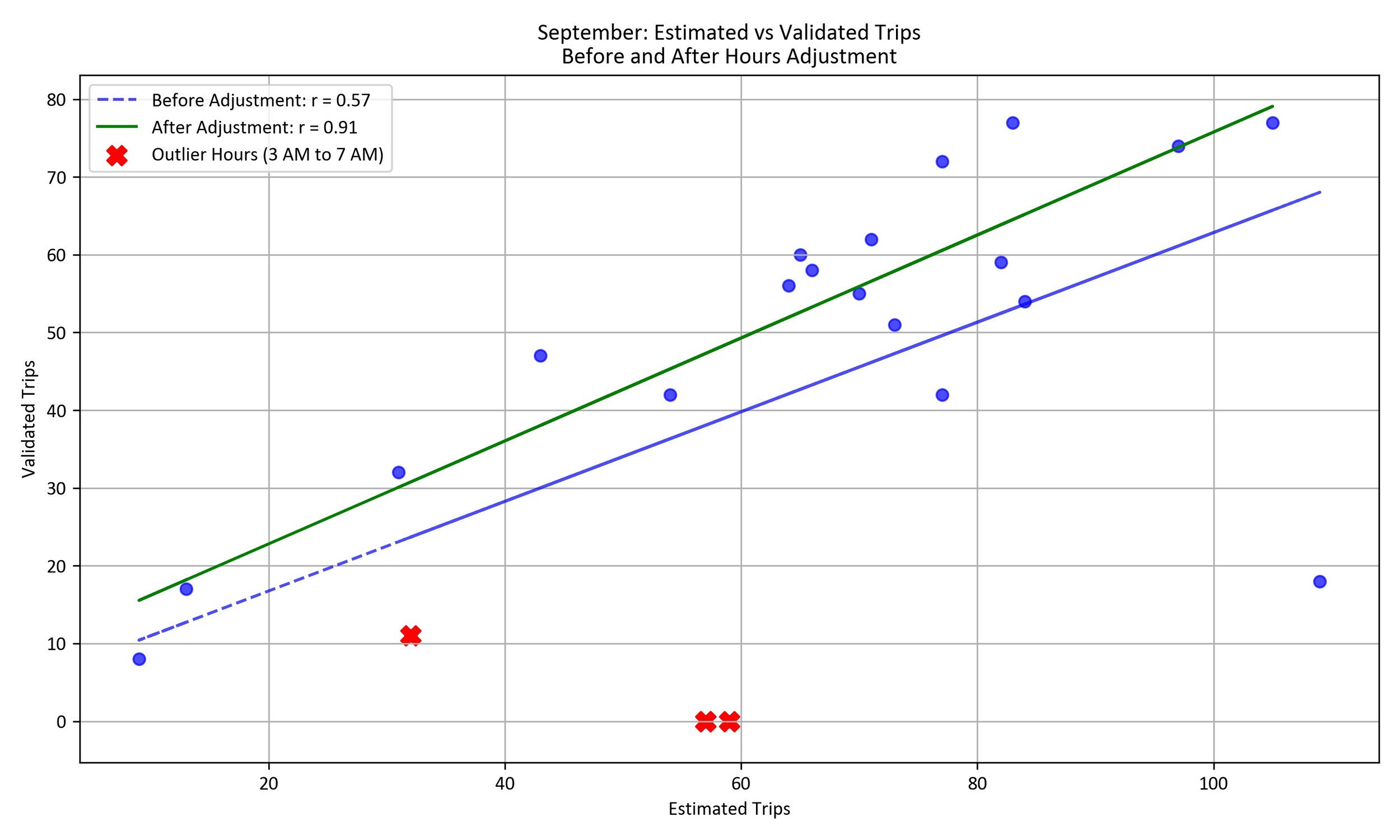
Figure 3 illustrates the estimated hourly trips by the algorithm vis-à-vis actual trips for a full month of data. The initial trip estimates (orange line) did not account for the time lag in GPS updates, where trips occurring in the final minutes of an hour were reported in the next hour, leading to rounding errors. Having had the advantage of obtaining actual trip O-D data, we fine-tuned the model through scaling, adjusting the estimates to account for the GPS time lag (green line), which greatly improved model performance. This refined model achieved a Mean Absolute Error (MAE) of 6.29, a Root Mean Squared Error (RMSE) of 7.85, and an R² (Coefficient of Determination) of 0.822, (with improvements from MAE=13.28, RMSE=16.91, and R2=0.822, respectively) indicating a much better fit between the estimated and observed trips. The significance of refinement by scaling is that, when validation data is available, scaling is preferable (green). However, in the most practical scenario (where validation data is absent), the unscaled model (orange) may be used.
_estimates_acros.jpg)
It should be noted that the primary emphasis of our validation is in the temporal dimension. We also attempted to validate the model spatially using Moran’s I and Geary’s C. Discrepancies between estimated and actual trip origins and destinations were randomly distributed (Moran’s I = -0.011, p-value = 0.191) with local variation (Geary’s C = 1.046, p-value = 0.007). The results of spatial validation, at best, are inconclusive.
To test the scalability of our algorithm, we applied the trip O-D estimation methodology developed using the data for the City of Fairfax to GBFS data in Washington, D.C., a much larger geography with higher trip density, diverse activity hubs, and broader geographic spread. The efficacy of this algorithm is demonstrated in Figure 4, which highlights the diurnal trip activity patterns for a single operator in Washington, D.C. The figure reveals that weekday trip activity is concentrated in the core business regions of downtown D.C., particularly during the midday and afternoon hours. In contrast, weekends see higher trip activity around the National Mall (not shown in the figure), reflecting shifts in leisure-related movement patterns. The model was able to accurately capture these dynamics, estimating a total of approximately 85,000 trips for the month of May 2021 for the single operator in D.C. By scaling the model to fit the unique spatial and temporal patterns of Washington, D.C., the approach effectively illustrated how trip production fluctuates between weekdays and weekends, with peaks during commute hours on weekdays and tourist-related activity during weekends.

The algorithm and methodology provide a reliable, portable, and scalable approach for understanding shared micromobility operations across multiple U.S. cities, without requiring data sharing agreements. The validation of our model across different cities highlights its adaptability and ability to accurately capture local trip patterns. Our methodology remains applicable to newer versions of GBFS specifications that have been released after 2021, the validation year. By utilizing real-time GBFS data from open-source APIs, stakeholders can evaluate system performance throughout the year, offering critical insights for various stakeholders, particularly regarding the feasibility of first- and last-mile solutions.
Further engagement with operators and fleet managers could enhance the model’s accuracy, especially during non-peak hours and for rebalancing trips. It’s also important to note that regional boundaries and rebalancing cycles may introduce over- or underestimation of trips due to GPS update lags, particularly near jurisdictional geofencing boundaries. Future research should focus on addressing these boundary effects to further refine the model’s accuracy in such conditions.