Loading [Contrib]/a11y/accessibility-menu.js
Skip to main content
null
Findings
  • Menu
  • Articles
    • Energy Findings
    • Resilience Findings
    • Safety Findings
    • Transport Findings
    • Urban Findings
    • All
  • For Authors
  • Editorial Board
  • About
  • Blog
  • covid-19
  • search

RSS Feed

Enter the URL below into your favorite RSS reader.

http://localhost:10836/feed
Transport Findings
October 31, 2024 AEST

Assessing the Impact of Distance Modelling Approaches on Active Travel Predictions

Laya Hossein Rashidi, Jennifer (L.) Kent, Emily Moylan,
Active traveldistance modellingpiecewise approachtravel behaviour
Copyright Logoccby-sa-4.0 • https://doi.org/10.32866/001c.125151
Findings
Hossein Rashidi, Laya, Jennifer (L.) Kent, and Emily Moylan. 2024. “Assessing the Impact of Distance Modelling Approaches on Active Travel Predictions.” Findings, October. https:/​/​doi.org/​10.32866/​001c.125151.
Save article as...▾
Download all (1)
  • Figure 1. Probability of active mode versus distance for each treatment of distance. All other variables are fixed at the mean (continuous) or mode (categorical).
    Download

Sorry, something went wrong. Please try again.

If this problem reoccurs, please contact Scholastica Support

Error message:

undefined

View more stats

Abstract

Trip distance is widely considered a key determinant of active travel choice, although distance is handled in choice modelling in various ways. This study examines how linear, categorical, quadratic, and piecewise representations for distance influence mode choice. The piecewise approach demonstrates superior fit and provides more stable elasticity estimates, ranging from -1% to -3%, compared to the broader range of -0.17% to -36% observed in categorical treatments and occasional positive values in quadratic treatments. These results underscore the piecewise model’s advantage in capturing critical behavioural shifts and offering more reliable insights to inform policy.

1. QUESTIONS

Active travel (AT) (i.e., walking and cycling) offers individual and community-wide benefits. For example, it fosters physical activity and social interaction and reduces car use (Faulkner et al. 2009; McDonald et al. 2016). While the determinants of active travel are complex, distance from origin to destination is a significant barrier to active travel, especially for younger populations, as they are sensitive to distance because of their small steps (Nelson et al. 2008). Despite its importance, there are multiple ways to model distance, and little consensus on which method is more accurate.

Many choice models employ distance as a continuous independent variable, assuming a direct relationship between distance and the utility of active travel (Mitra, Buliung, and Roorda 2010), which may oversimplify complex behavioural patterns. Since the utility is exponentiated via a logistic function in logit models, the linear treatment of distance does not suggest a linear decrease in the probability of choosing active mode. Categorical treatments divide distance into specific bands, such as 0-1 km and 1-2 km, to capture distinct travel behaviour patterns (Mitra and Buliung 2015). While this approach recognises that shorter distances may encourage active travel, sharp category boundaries can lead to misleading interpretations, particularly at the breakpoints, and are insensitive to the impact of distance within the same category. Quadratic approaches, on the other hand, offer flexibility by capturing non-linear effects, but can complicate result interpretation with higher-order terms (Subhojit 2021).

Finally, there are piecewise approaches, which divide distance variable into distinct intervals, allowing each interval to have a separate coefficient while maintaining continuity at the breakpoints (Train 2009). By doing so, piecewise treatment of distance can capture critical behavioural shifts, such as a sharp decline in walking or cycling beyond a certain distance, offering superior accuracy.

The key question addressed in this paper is whether piecewise treatments address the limitations of linear, logit, quadratic, and categorical approaches in explaining active modes. Using a database of 7555 students’ journeys to school from Sydney, Australia, the study compares different methods to assess distance’s impact on model fit, active mode probability predictions across distance ranges, and distance elasticity estimates.

2. METHODS

The study utilises data from the 2015 School Physical Activity and Nutrition Survey (SPANS), which includes detailed attributes such as age, gender, socioeconomic status (SES), school type, and travel mode choice (as detailed in Hardy et al. (2017). Built-environment measures, including population density (ABS 2016b), land-use mix (ABS 2016a), intersection density (Geofabrik 2018), cycling infrastructure (Open data hub 2023), and traffic calming (Geofabrik 2018), were also appended, based on the school location. Table 1 provides the description of the variables used.

Table 1.Descriptive analysis of variables of the study.
Variable Description Source Mean (SD)
Mode Active=1, motorised=0 SPANS 0.2 (0.4)
Age Age SPANS 10.2 (3.3)
Female Gender (Female=1, otherwise=0) SPANS 0.5 (0.5)
English English (as a first language) = 1, otherwise =0 SPANS 0.9 (0.3)
SES Socio Economic Status score (/1000) SPANS 1.0 (0.1)
Regional Live in regional or remote areas=1, otherwise = 0 SPANS 0.2 (0.4)
Gov Study in Government school =1, otherwise =0 ACARA 0.6 (0.5)
Dist Distance (km) Imputed from SPANS 4.9 (4.1)
Dist_square Distance * distance (km2) SPANS 40.5 (62.2)
Dist_0_=1km_dm Distance less than 1km = 1, otherwise = 0 SPANS 0.1 (0.3)
Dist_1_=3km_dm Distance between 1-3km = 1, otherwise =0 SPANS 0.3 (0.5)
Dist_3_=5km_dm Distance between 3-5km = 1, otherwise = 0 SPANS 0.1 (0.3)
Dist<=1km_PW Piecewise distance between 0-1km SPANS 0.9 (0.2)
Dist_1_=3km_ PW Piecewise distance between 1-3km SPANS 1.4 (0.8)
Dist_3_=5km_ PW Piecewise distance between 3-5km SPANS 1.0 (1.0)
Dist>5km_ PW Piecewise distance more than 5km SPANS 1.6 (2.9)
Popdens Population density (1000 people/km2) ABS 8.8 (7.2)
LU-mix Land-use mix (Entropy index) ABS 0.5 (0.1)
Bike-lane Bike lane length density (1/km) Open data hub 2.5 (1.7)
Intersect Intersection density (100/km2) Geofabrik 5.7 (3.8)
Traff-calm Stop sign and traffic signal (1/km2) Geofabrik 5.1 (6.5)

Five binary choice models were developed to assess how distance affects the likelihood of choosing between active versus non-active travel modes. The models vary only in their treatment of distance: no distance variable, linear, quadratic, categorical, and piecewise specifications. Control variables included demographic and built-environment factors.

Model estimation was performed using the Biogeme package (Bierlaire 2009), with performance assessed through McFadden’s R2, and Akaike Information Criterion (AIC). Elasticity values, representing the percentage change in active mode choice probability for a one per cent increase in distance, were computed and summarised across demographic segments to highlight the implications for different population groups.

3. FINDINGS

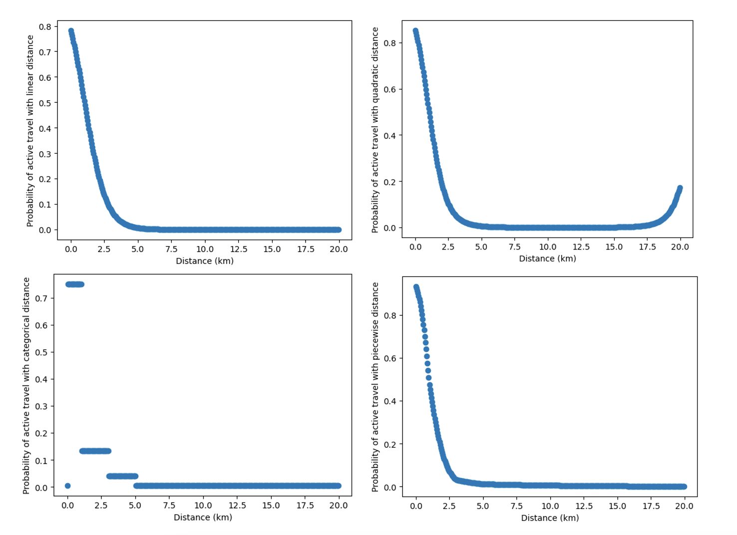
The piecewise model demonstrates the best overall fit among the five models, as indicated by the highest McFadden’s R2 value (66%) and the lowest AIC (3128.2) score, as illustrated in Table 2. While the linear, quadratic, and categorical models also perform well, their fit metrics are slightly lower compared to the piecewise model. In the piecewise model, the negative coefficients for each distance range emphasise the sharp decline in active travel likelihood as distance increases (e.g., -2.73 within the first cap). This suggests that the negative relationship between active travel and distance changes substantially in magnitude at certain thresholds. Based on this evidence, the linear specification not only reduces the model’s predictive power but also overlooks the non-linear behaviour. Thus, the linear specification is not recommended for use in this context.

Table 2.The comparison of binary logit models of being active using different types of distance. Piecewise distance, which reflects the non-linearity impact of distance, has the best goodness of fit.
Variables Without Linear Quadratic Categorical Piecewise
Constant -4.61*** -1.19 -0.54 -7.34*** 0.26
Age 0.02 0.11*** 0.12*** 0.16*** 0.13***
Female -0.20*** -0.30*** -0.30*** -0.30*** -0.31***
SES 1.91*** 0.72 0.45** 0.17 0.41
English -0.14 -0.30** -0.32** -0.43*** -0.35**
Regional 0.05 0.72*** 0.76*** 0.76*** 0.84***
Government 1.31*** 0.55*** 0.54*** 0.63*** 0.56***
Distance - -1.26*** -1.77*** - -
Dist_square - - 0.08*** - -
Dist_0_1km_dmy - - - 6.33*** -
Dist_1_=3km_dmy - - - 3.36*** -
Dist_3_=5km_dmy - - - 2.05*** -
Dist<=1km_PW - - - - -2.73***
Dist_1_=3km_PW - - - - -1.65***
Dist_3_=5km_PW - - - - -0.50***
Dist>5km_PW - - - - -0.15*
Popdens 0.04*** 0.05*** 0.05*** 0.04*** 0.05***
LU-mix -0.04 0.17 0.23 0.16 0.19
Bike-lane 0.05** 0.10*** 0.11*** 0.12*** 0.12***
Intersection -0.05*** -0.05*** -0.05*** -0.05*** -0.05***
Traff-calm 0.03*** 0.03*** 0.03*** 0.02*** 0.03***
Sample size 6478 6478 6478 6478 6478
Null log likelihood -4490.2 -4490.2 -4490.2 -4490.2 -4490.2
Final log likelihood -2953.0 -1699.0 -1595.0 -1657.7 -1548.1
McFadden’s R2 0.34 0.62 0.64 0.63 0.66
AIC 5929.9 3424.0 3217. 9 3345.3 3128.2

* p<.1, ** p<.05, ***p<.01

Walking probability versus distance plots show a discontinuity in the walking probability at the breakpoints of the categorical model, which is counterintuitive (Figure 1). However, the other models display a more logical trend, albeit with different gradients. The quadratic model shows an unexpected incline at longer distances, suggesting an increase in walking probability beyond 18 km, which is implausible. This anomaly arises from the second power of distance, which corrects for non-linearity at shorter distances but produces unrealistic results at larger distances. These probability plots suggest that categorical variables and quadratic forms should be avoided, especially when travel distances, including non-walking modes, can be large, as is often the case in a city like Sydney.

Figure 1
Figure 1.Probability of active mode versus distance for each treatment of distance. All other variables are fixed at the mean (continuous) or mode (categorical).

Mean elasticity values in Table 3 compare the estimated elasticities across three dimensions: Location (Inner Regional, Major Cities, Outer Regional, Remote), SES (low: <800, mid: between 800 and 1000, high: >1000), and distance bands (0-1km, 1-3km, 3-5km, >5km). The average distance elasticity shows a consistent elasticity of about -2% across quadratic, categorical, and piecewise models, while the linear model shows -4.6%. This discrepancy is more pronounced for certain subgroups; for example, in Inner Regional areas with low SES and 3-5 km, the linear, quadratic, categorical, and piecewise models yield elasticities of -5%, -4%, 0, and -2%, respectively. Such significant differences are concerning, particularly when using elasticity values for policy assessments, including equity-based interventions targeting specific demographic groups. Additionally, piecewise elasticities tend to be more stable, generally ranging from -1% to -3%, whereas the categorical model exhibits a broader range from -0.17% to -36%. Quadratic elasticities occasionally show positive values, which is counterintuitive but consistent with earlier observations from probability versus distance plots.

The influence of the built-environment on active transport is complex. While these findings are limited to a specific built and cultural context, they do underscore the importance of model specification in understanding and promoting active travel. Future research is required to apply these findings to other contexts and modes. Nevertheless, it is clear that piecewise models offer a more accurate reflection of distance effects, supporting their use in research and interpretation into policy outcomes.

Table 3.Comparison of elasticity analysis of ATS to different forms of distance among different demographic segments.
Location SES tertile Distance (km) Linear Quadratic Categorical Piecewise
Inner Regional high >5 -14.63 5.93 0 -1.86
Inner Regional high 1-3 -1.83 -1.99 -36.37 -2.45
Inner Regional high <1 -0.13 -0.14 0 -0.14
Inner Regional low >5 -10.90 -0.65 0 -1.35
Inner Regional low 3-5 -4.76 -4.22 0 -1.91
Inner Regional low 1-3 -1.95 -2.19 -2.54 -2.73
Inner Regional low <1 -0.14 -0.15 0 -0.20
Inner Regional mid >5 -10.35 -1.36 -0.19 -1.29
Inner Regional mid 3-5 -4.749 -4.23 -2.35 -1.91
Inner Regional mid 1-3 -2.11 -2.36 -6.47 -2.94
Inner Regional mid <1 -0.18 -0.20 0 -0.27
Major Cities high >5 -10.04 -1.26 -0.36 -1.25
Major Cities high 3-5 -4.71 -4.23 -1.50 -1.91
Major Cities high 1-3 -2.00 -2.27 -10.4 -2.797
Major Cities high <1 -0.22 -0.27 0 -0.37
Major Cities low >5 -10.56 -0.83 -0.17 -1.32
Major Cities low 3-5 -4.67 -4.21 0 -1.88
Major Cities low 1-3 -2.33 -2.59 -2.67 -3.19
Major Cities low <1 -0.22 -0.26 0 -0.35
Major Cities mid >5 -10.28 -1.25 -0.17 -1.28
Major Cities mid 3-5 -4.75 -4.23 -1.10 -1.92
Major Cities mid 1-3 -1.93 -2.19 -9.04 -2.70
Major Cities mid <1 -0.21 -0.24 0 -0.35
Outer Regional low >5 -11.02 -0.64 0 -1.37
Outer Regional low 3-5 -4.43 -4.08 -5.76 -1.80
Outer Regional low 1-3 -1.94 -2.18 -12.16 -2.71
Outer Regional low <1 -0.20 -0.23 0 -0.31
Outer Regional mid >5 -10.20 -1.96 0 -1.24
Outer Regional mid 3-5 -4.69 -4.12 0 -1.88
Outer Regional mid 1-3 -1.58 -1.79 0 -2.26
Outer Regional mid <1 -0.16 -0.17 0 -0.25
Remote low >5 -12.39 -0.77 0 -1.55
Remote mid >5 -9.07 -2.63 0 -1.12
Remote mid 3-5 -4.84 -4.29 -2.20 -1.95
Remote mid 1-3 -2.35 -2.62 -8.82 -3.19
Remote mid <1 -0.26 -0.30 0 -0.39
Total Total Total -4.63 -1.70 -1.70 -1.57

ACKNOWLEDGMENTS

This study used the SPANS dataset, funded by the NSW Ministry of Health. We also acknowledge the SPANS data collection team and are particularly thankful to Dr Louise Hardy for her assistance with this work. Finally, we acknowledge the students, parents, schools and staff who participated.

This research is supported by an Australian Government Research Training Program (RTP) Scholarship and the Australian Research Council (DE190100211).

Submitted: September 25, 2024 AEST

Accepted: October 26, 2024 AEST

References

ABS. 2016a. “Australian Statistical Geography Standard (ASGS): Volume 1—Main Structure and Greater Capital City Statistical Areas.” https:/​/​www.abs.gov.au/​AUSSTATS/​abs@.nsf/​DetailsPage/​1270.0.55.001July%202016?OpenDocument.
———. 2016b. “TableBuilder.” Australian Bureau of Statistics. 2016. https:/​/​www.abs.gov.au/​websitedbs/​censushome.nsf/​home/​tablebuilder.
Bierlaire, M. 2009. Estimation of Discrete Choice Models with BIOGEME 1.8.
Google Scholar
Faulkner, G. E. J., R. N. Buliung, P. K. Flora, and C. Fusco. 2009. “Active School Transport, Physical Activity Levels and Body Weight of Children and Youth: A Systematic Review.” Preventive Medicine 48 (1): 3–8. https:/​/​doi.org/​10.1016/​j.ypmed.2008.10.017.
Google Scholar
Geofabrik. 2018. “Geofabrik Download Server.” 2018. http:/​/​download.geofabrik.de/​australia-oceania/​australia.html.
Hardy, L. L., S. Mihrshahi, B. A. Drayton, and A. E. Bauman. 2017. “NSW Schools Physical Activity and Nutrition Survey (SPANS).” NSW Department of Health. https:/​/​ses.library.usyd.edu.au/​handle/​2123/​16754.
McDonald, N. C., R. L. Steiner, W. M. Palmer, A. N. Bullock, V. P. Sisiopiku, and B. F. Lytle. 2016. “Costs of School Transportation: Quantifying the Fiscal Impacts of Encouraging Walking and Bicycling for School Travel.” Transportation 43 (1): 159–75. https:/​/​doi.org/​10.1007/​s11116-014-9569-7.
Google Scholar
Mitra, R., and R. N. Buliung. 2015. “Exploring Differences in School Travel Mode Choice Behaviour between Children and Youth.” Transport Policy 42:4–11. https:/​/​doi.org/​10.1016/​j.tranpol.2015.04.005.
Google Scholar
Mitra, R., R. N. Buliung, and M. J. Roorda. 2010. “Built Environment and School Travel Mode Choice in Toronto, Canada.” Transportation Research Record 2156 (1): 150–59. https:/​/​doi.org/​10.3141/​2156-17.
Google Scholar
Nelson, N. M., E. Foley, D. J. O’Gorman, N. M. Moyna, and C. B. Woods. 2008. “Active Commuting to School: How Far Is Too Far?” International Journal of Behavioral Nutrition and Physical Activity 5 (1): 1. https:/​/​doi.org/​10.1186/​1479-5868-5-1.
Google Scholar
Open data hub. 2023. “Datasets | TfNSW Open Data Hub and Developer Portal.” Open Data. 2023. https:/​/​opendata.transport.nsw.gov.au/​search/​type/​dataset.
Subhojit, R. 2021. “Threshold Value Estimation of Journey-Distance Using Generalized Polynomial Function.” European Transport/Trasporti Europei, 1–17. https:/​/​doi.org/​10.48295/​ET.2021.84.3.
Google Scholar
Train, K. 2009. “Discrete Choice Methods With Simulation.” In Discrete Choice Methods with Simulation, Second Edition. Vol. 2009. https:/​/​doi.org/​10.1017/​CBO9780511805271.
Google Scholar

This website uses cookies

We use cookies to enhance your experience and support COUNTER Metrics for transparent reporting of readership statistics. Cookie data is not sold to third parties or used for marketing purposes.

Powered by Scholastica, the modern academic journal management system