1. Question
Location-based services (LBS) data contain the spatial locations of many mobile phone users, but they do not independently describe travel behavior (Du and Aultman-Hall 2007). A classification of the LBS data from raw location points to semantic activities is potentially desirable for many reasons, including removing error from travel diaries, improving the quality of travel models, and providing insights into traveler decisions (Bohte and Maat 2009; Usyukov 2017).
The most basic attempts have used heuristic algorithms. Common heuristics include the implied speed between points, or direction between series of points (Deng and Ji 2010). But it is difficult to develop conclusive rules: is a person moving slowly because they are waiting for a traffic signal or because they are doing an activity? Decision trees can expand the number and types of rules (Lee and Lee 2014), potentially increasing the classification accuracy. More advanced methods rely on artificial intelligence (AI), but these can be difficult to deploy at smaller scales, or to train from unlabeled data (Xiao, Juan, and Zhang 2016); it is not clear in the literature how many labeled user-days would be necessary to train the AI. An intermediate approach of density-based clustering algorithms (Duan et al. 2007; Gong, Yamamoto, and Morikawa 2018; Luo et al. 2017) shows promise for particular applications where a neural network may be difficult to train. But these methods require estimating or asserting parameters that may not be immediately intuitive.
In this research, we develop an error function describing the accuracy of activity locations classified by a Density-Based Spatial Clustering with Additional Noise and Time Entropy (DBSCAN-TE) algorithm. We calibrate the algorithm’s parameters by optimizing the function against manually-labeled activity locations.
2. Methods
2.1. DBSCAN-TE Algorithm
The DBSCAN-TE algorithm classifies activities from raw location data in two steps. First, a DBSCAN clustering algorithm (Rehman et al. 2014) finds high-density areas in the spatial data and excludes noise. This algorithm requires two parameters: the radius of an activity cluster; and the minimum number of cluster points
The second step is a time and entropy step. DBSCAN alone cannot distinguish between clusters that are separated by time and not space. For example, individuals may begin their day at home and return later; DBSCAN classifies both sets of points as one activity, because they are at the same location. A time parameter is used to separate LBS point in the same cluster that are at least units apart. Finally, DBSCAN-TE considers the “entropy” of points within a candidate cluster, where entropy is a function of the directions between consecutive LBS data points. This eliminates clusters where the device is slowly moving in one direction — as in a traffic queue. The angle between consecutive points is mapped onto sectors of a circle, and then the entropy is calculated as :
S=−D∑d−1ndNln(ndN)
where is the number of directions falling in sector is the total number of rays in the cluster, and is the total number of sectors (often (Gong, Yamamoto, and Morikawa 2018). If (a set threshold), then that cluster is disqualified as an activity point.
2.2. Error Measurement and Calibration
We desire to identify the parameters vector that minimizes the “error” between activity points generated by DBSCAN-TE and labeled activity points for a user-day. Let be the set of location points for a user-day is the set of points within a distance of a labeled activity point on the user day and as the set of points within the same distance of an activity point identified by DBSCAN-TE. The total error is
E=N∑i=1[1−|Li∩Di|+|Pi∖(Li∪Di)||Pi|]
where are the points in both the labeled data and the predicted data, and are the points assigned to an activity cluster in neither. Thus the error for a user-day is effectively the share of points that are differently classified by and The total error is the sum of this value for all user days.
To identify parameters minimizing the error functions, we use a simulated annealing algorithm in R (King, Nguyen, and Ionides 2016). Simulated annealing is useful in finding global optima on non-convex or discontinuous objective functions (Bertsimas and Tsitsiklis 1993). Simulated annealing also permits box constraints on the parameters and parameter scaling: are defined on different scales with different units. The constraint values are shown in Table 1 values and were set based on an initial search of the literature (Duan et al. 2007; Gong, Yamamoto, and Morikawa 2018; Luo et al. 2017) supported by intuition. For example, we set a minimum minutes (300 seconds), believing a gap this short to be an unrealistic duration for an intervening activity. The scale parameters were set so that the range covered by the parameters was similar across all four dimensions.
2.3. Data
Data for this study come from a comprehensive longitudinal dataset of 78 volunteers using a mobile application that collects detailed location-based services data. We drew a random sample of 25 high-quality user-days — defined as 24 hours between 3 AM and 2:59 AM the next day, having a time density of location points of at least 30 points per minute. We mapped the points in GIS software and manually added points at the visually apparent activity locations.
3. Findings
We ran the simulated annealing algorithm for 5000 iterations, beginning with four randomly sampled sets of starting values. Table 2 shows the results of each run alongside a mean value. For most parameters, there is some level of agreement on the scale of the parameters, with three of the four runs matching in the first or second significant digit. The anomalous value differs between runs however, as Run 3 has a low and Run 4 a low The mean error of 1.29 implies the algorithm predicts 94.9 percent of points correctly across the 25 user-days.
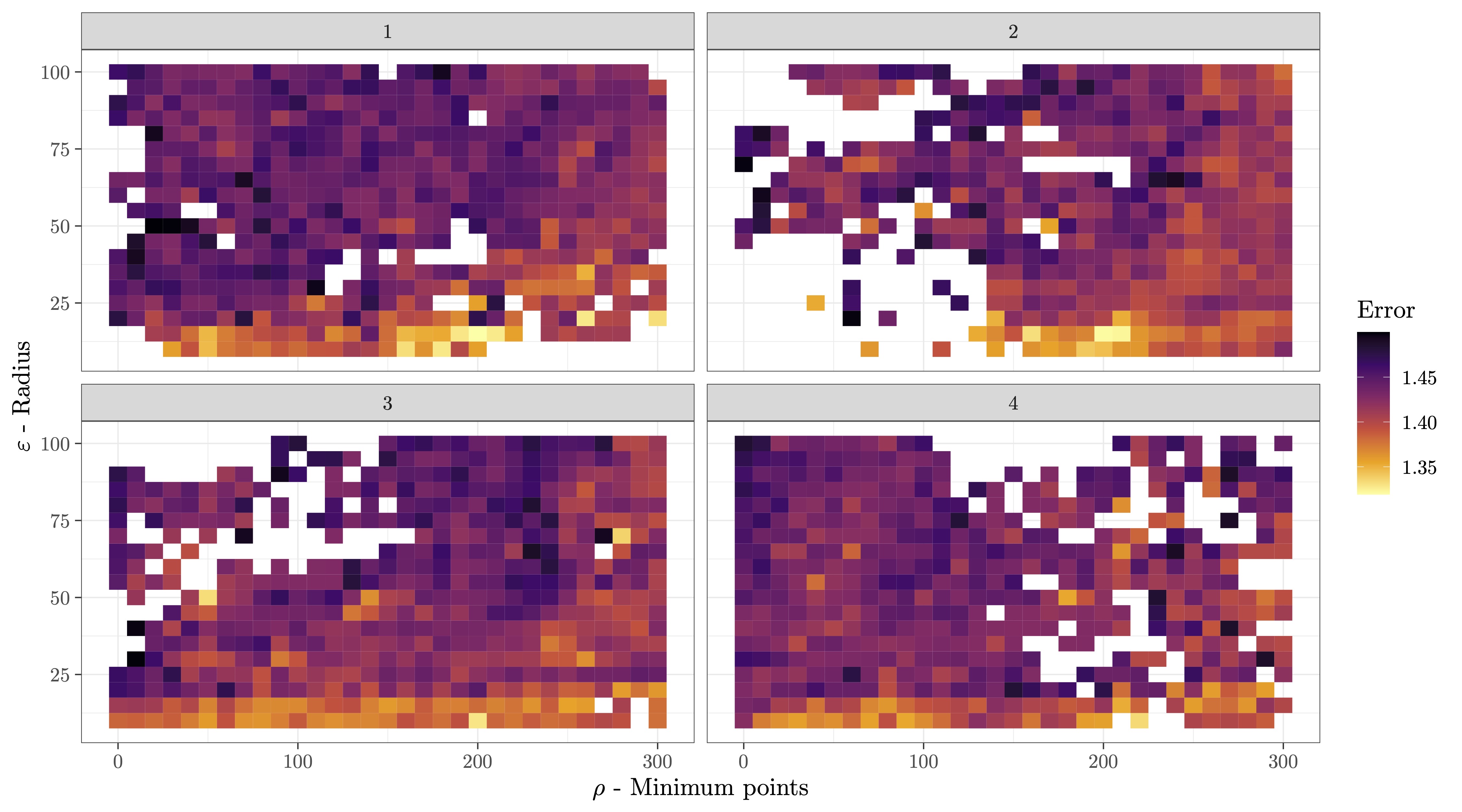
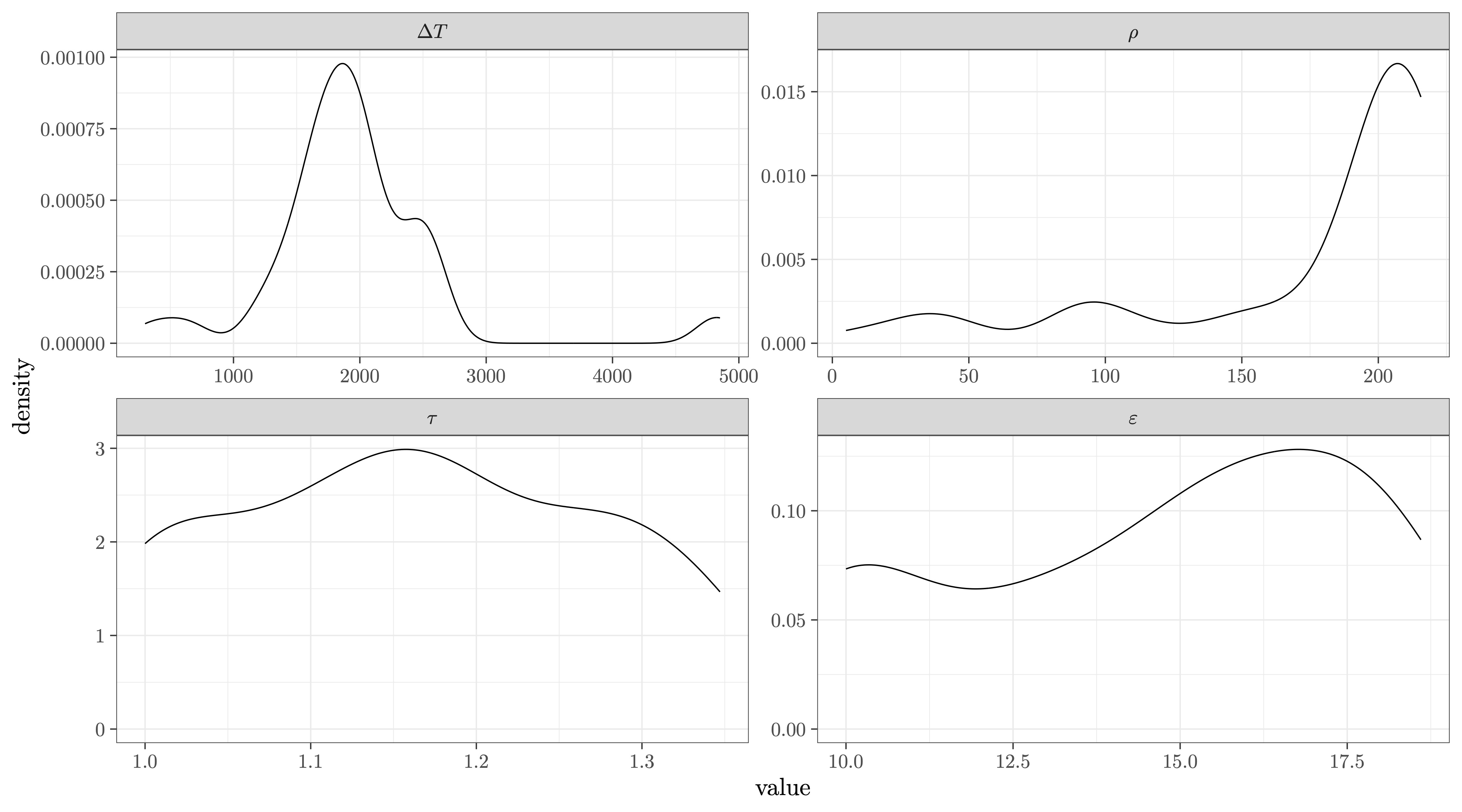
Figure 1 shows the mean value of the error function across the parameters If a cell is blank, then the simulated annealing algorithm did not search there, or the error exceeded 1.5. This figure only shows two dimensions of the four in the objective function, so there is variance at each coordinate. Nevertheless, the plot shows consistently lower error for low and Figure 2 shows a density of each parameter across all four runs with The results of 55 iterations are included. The distribution is weighted by the inverse error, with an index for the optimization iteration. Other weight constructions did not result in substantially different interpretations of this figure. The modes of this density plot are candidates for the preferred values.


Researchers with unlabeled location-based services data may use the DBSCAN-TE algorithm directly using the parameters identified in this research, but should exercise caution. The most sensitive parameter in other data sets is likely to be the minimum points to constitute a cluster: with less temporally dense data, fewer points will accumulate and the 200 point threshold may not be a viable option. Understanding the relationship between data density and the values of these parameters is important future research.
A different error function could be developed that includes not only the location but the duration of activities, and their sequence in a time-space framework. This would improve the accuracy of the calibration but also increases the difficulty of the labeling task. Similarly, data with a different temporal or spatial resolution may lead to different optimal parameters. Further research should also explore how many labeled user-days are sufficient to identify stable parameters in the DBSCAN-TE algorithm versus train an AI to perform this task accurately.
Acknowledgments
This data used in this research was collected with help from an Interdisciplinary Research Grant at Brigham Young University, and administered under IRB protocol F2020-242. The investigators on the overarching grant include Terisa Gabrielsen, Jared Nielsen, and Mikle South. Myrranda Salmon supported the data cleaning efforts.
Author Contribution Statement
Gregory S. Macfarlane: Conceptualization, Methodology, Software, Formal Analysis, Writing - original draft, Supervision Gillian Martin: Methodology, Software, Investigation, Writing - original draft Emily K. Youngs: Software, Formal Analysis, Data curation Jared A. Nielsen: Resources, Writing - review & editing, Supervision, Project administration, Funding acquisition