Where to Put Bike Counters? Stratifying Bicycling Patterns in the City Using Crowdsourced Data

1. RESEARCH QUESTION AND HYPOTHESIS

When a city aims to quantify bicycling volume, data are typically collected at a sample of locations via manual counts and automatic counters (Griffin et al. 2014; Nordback et al. 2013). The goal is to select locations for bicycle volume counting that are representative of volumes throughout the city. Systematic approaches that utilize fine spatial and temporal resolution crowdsourced data have the potential to improve sampling efficiency and representativeness for bicycle counts.

New bicycling ridership data, which are continuous across space and time, are available from crowdsourced tools (i.e., Strava) and provide an opportunity to develop methods to stratify sampling when locating count stations. Strava’s data provide the number of app users on a street segment every minute and, despite a bias toward leisure bicycling, have been shown to moderately correlate with overall bicycling ridership (Jestico, Nelson, and Winters 2016; Boss et al. 2018). Strava can be used to differentiate high- and low-volume streets, as well as streets used during peak commute times. Streets with similar ridership patterns can be categorized, and these categories can be used as factors to stratify field- and volunteer-based bicycling volume counter programs to obtain more precise information (Nordback et al. 2019).

We used crowdsourced data on bike ridership and continuous signal processing data mining to classify street segments by the temporal patterns in ridership. These were demonstrated in a case study of bicycling patterns in Ottawa, Ontario, Canada.

2. METHODS AND DATA

Strava Metro provided bicyclist counts for 2016 at one-minute temporal resolution for a 20 km² area in downtown Ottawa, where correlation coefficients between daily total counts from Strava and automated counters ranged from 0.76–0.96 (Boss et al. 2018). In order to obtain temporal profiles of bicycling ridership, we computed the average hourly activity count for bicycling on weekdays during nonwinter months (March–September) for each hour of the day for the 3,880 non-zero-count street segments.

To quantify the differences between bicycling ridership profiles of all street segments, we computed dynamic time warping (DTW) distances. DTW finds the optimal global alignment between two time series by computing a pairwise distance matrix (M) for all points in both time series (Equation 1) and by finding the least-cost path in M (Sakoe and Chiba 1978).

$$D = \left| A_{i} - B_{j} \right| + min\left\{ \left. \ \begin{matrix} D\ \lbrack i - 1,\ j - 1\rbrack \\ D \left\lbrack i - 1,\ j \right\rbrack \\ D\ \lbrack i,\ j - 1\rbrack \\ \end{matrix} \right\} \right.\ $$

Equation 1

Here $A_{i}$ is the mean cyclist count for street segment $A$ at hour $i$ , $B_{j}$ is the mean cyclist count for street segment $B$ at hour $j$, $D\ \lbrack i - 1,\ j - 1\rbrack$ is the previously computed difference between mean cyclist counts in the previous hour for both time series, $D\ \left\lbrack i - 1,\ j \right\rbrack$ is the previously computed difference between mean cyclist counts at the current hour for series $B$ and the previous hour for series $A$, and $D\ \lbrack i,\ j - 1\rbrack$ is the previously computed difference between mean cyclist counts at the current hour for series $A$ and the previous hour for series $B$.

We used a Sakoe-Chiba band (Sakoe and Chiba 1978) to constrain warping to a three-hour interval centered at the hour being warped to avoid unrealistic least-cost paths (Zhang et al. 2017). Pairwise distances yielded by the least-cost path were used to generate a 3,880 by 3,880 matrix (W) accounting for the differences among all bicycling ridership profiles.

In order to group street segments with similar bicycling ridership patterns, we applied Ward’s hierarchical bottom-up clustering algorithm to the W matrix of time series data (no spatial relationships in the road network data were used in the clustering). The algorithm starts with each street segment as its own group and successively merges them into clusters based on the minimum increase in the error sum of squares (Murtagh and Legendre 2014). We used the Calinski-Harabasz Index (CHI) (Calinski and Harabasz 1974) to select the optimal number of clusters. CHI considers the dispersion within and between groups; higher values indicate a better partition (Ahmed 2012).

We varied the number of clusters from 1–50 (more clusters than is practical to interpret) and selected the configuration with the highest CHI. We plotted the profiles within each cluster and analyzed their main characteristics to assign labels that are interpretable by city planners.

3. FINDINGS

Figure 1 shows the temporal profiles of ridership for all street segments in our study area. Similar profiles have been generated from single bicycling counters (Miranda-Moreno et al. 2013), but using Strava allows rich spatial resolution (every single street segment) in concert with the temporal richness. While Strava provides data based on only a sample of riders and there are demographic biases in the app users, research has shown the spatial patterns in this ridership data correlate with overall bicycle ridership volumes (Jestico, Nelson, and Winters 2016; Boss et al. 2018).

Figure 1:Weekday Average Temporal Profiles of Bike Ridership for all Street Segments in the Study Area for Nonwinter Months (March–September)

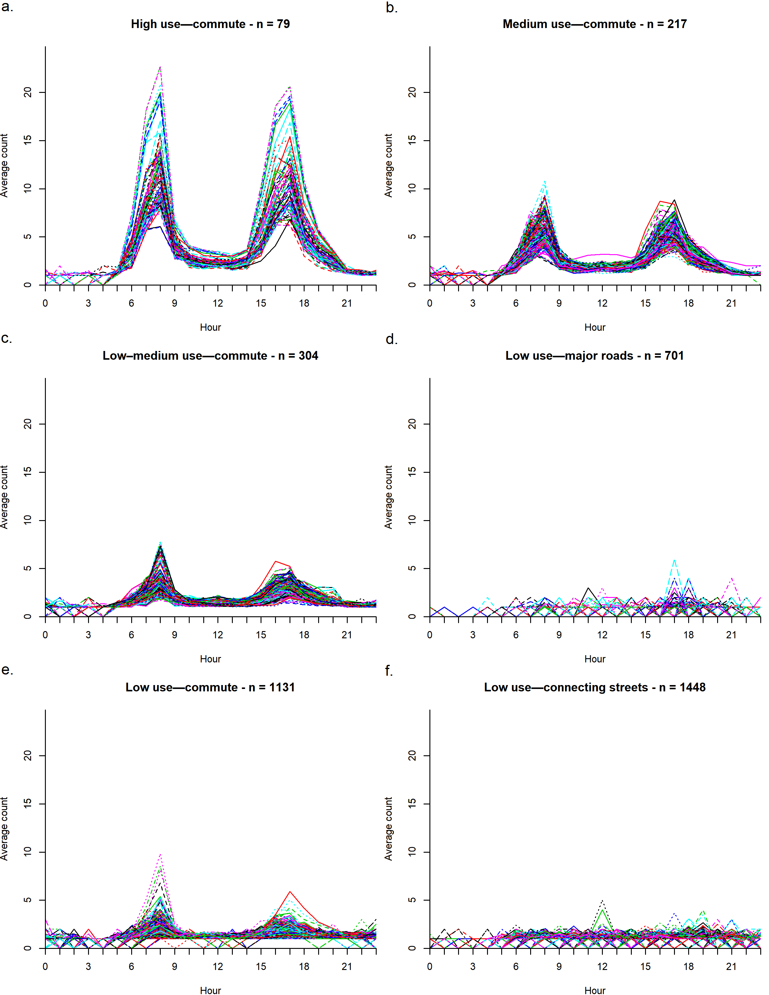
Figure 2 shows the temporal profiles for street segments within each bicycling ridership class identified by the clustering algorithm. We identify patterns of ridership and differences in volume (Figures 2a–d). The pattern we label as commute is characterized by two peaks (approximately 8:00 a.m. and 6:00 p.m.) with the maximum average volume of bicyclists varying from 25 (high use) to 5 (low use) at peak times. Figures 2e and 2f show the low-use classes, in which bike ridership is sporadic and the average volume of bicyclists is no higher than 5.

Figure 2:Bike Ridership Temporal Profiles for Street Segments within Each Bike Ridership Class

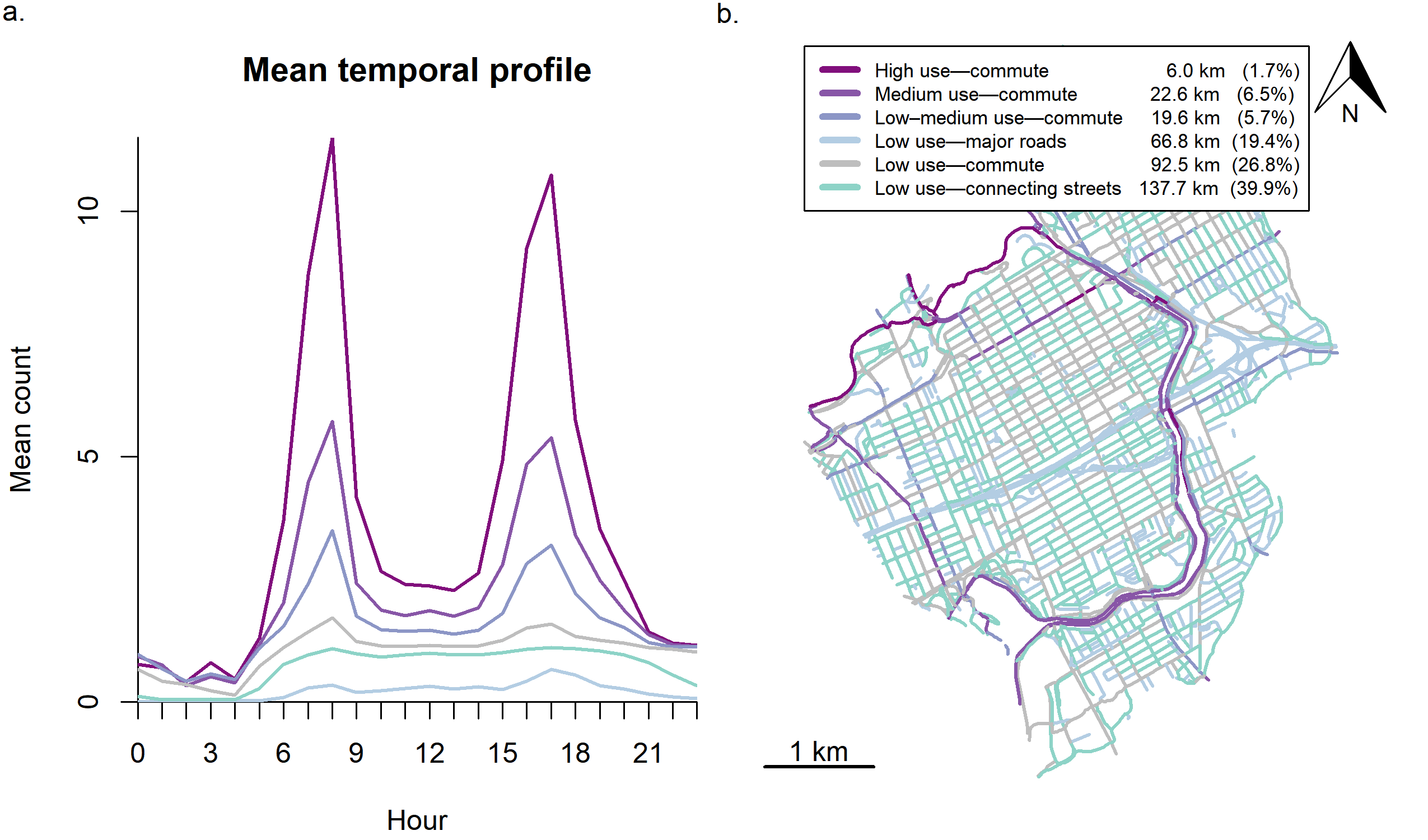
Figure 3 shows the mean temporal profile for each ridership class (a) and the spatial distribution of these classes (b). Street segments with high and medium commute volumes are along the Ottawa River, the Rideau Canal, the Trillium Pathway, and Laurier Avenue West. While the clusters had similar temporal patterns, differentiating classes by magnitude was useful for an end goal of stratified sampling.

Figure 3:a) Mean Temporal Profiles for the Classes of Bike Ridership; b) Map of Bike Ridership Classes for Study Area in Ottawa

Using crowdsourced bicycling data and continuous time-series processing allowed us to map street segments into classes of temporal patterns of bicycle ridership that can be used for targeted interventions and stratifying count programs. Ridership classes can help planners determine the most appropriate locations and times to obtain bicycle volume counts that are representative of ridership across the city. We recommend placing four or more counters per bicycling ridership class to maximize the precision of bicycling volume estimates (Nordback et al. 2019) and at least 50 counters for a medium-sized city (Roy et al., Forthcoming). This method is a novel systematic approach based on spatially and temporally detailed crowdsourced data to determine where bicycle counts should be sampled to efficiently collect representative data.

ACKNOWLEDGMENTS

The authors would like to acknowledge Strava and the city of Ottawa for providing the data. This work was supported by a grant from the Public Health Agency of Canada to BikeMaps.org.