RESEARCH QUESTION AND HYPOTHESIS

Vehicle-miles traveled (VMT) or vehicle-kilometers (km) travelled (VKT) is a key measure of household travel behaviors and, therefore, regional and interregional travel demand (Cervero and Hansen 2002). Single-day and two-day travel surveys are the norm, with households completing detailed trip diaries and providing vehicle odometer values for 24- to 48-hour durations. Individuals and their households travel patterns, however, can vary considerably over time (Pendyala and Pas 2000). This day-to-day and month-to-month variability differs across households, drivers, and their vehicles. To reduce uncertainty in vehicle travel estimates by being more strategic in determining sample sizes and survey durations across demographic and other strata, this article explores day-to-day variability in vehicles tracked for an entire year of driving. The work investigates how valuable one-day versus two-day versus seven-day data are for inferring a year’s worth of driving behaviors and which persons and household types tend to offer the most stable versus variable driving patterns, across days of the year.

METHODS AND DATA

The data used here comes from the Puget Sound Regional Council’s Traffic Choices Study (NREL 2017), for the Seattle region of Washington in the United States. The data was collected between November 2004 and August 2006 by placing GPS tolling meters on the vehicles of volunteer households. The final data set contains 329 unique households and 484 vehicles. The duration of GPS device placement on vehicles varied across households and across vehicles within each household. In this study, vehicles with less than a full year (365 days) of data were excluded. To avoid correlations in travel between pairs or triplets of vehicles owned by the same household, only one vehicle per household has been randomly selected for analysis.

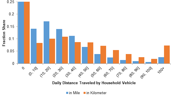
Figure 1 provides histograms of daily VMT and VKT values for all 252 vehicles. Common values are zero-kilometer days (25% doing no driving on that GPS-survey day), and between 16.1 and 32.2 km (10 and 20 miles) per day (17.1%). Average daily travel is 38.9 ± 55.8 km (24.2 ± 34.7 miles) per vehicle, which is reasonably consistent with the average daily vehicle travel of 46.62 km (28.97 miles) per day per driver, as found in the 2009 National Household Travel Survey (NHTS) (Santos et al. 2011).

Figure 1:Histogram for Daily VMT and VKT (N= 91,980 survey days, across 252 household vehicles)

A total of 60 runs of regression were made, with 20 different sets of starting dates for all vehicles randomly selected and the short period capturing one, two, or seven days of travel data, respectively. Table 1 shows adjusted R² values of all 60 ordinary least squares (OLS) regressions, which increase as the sampled length is extended. An entire week’s data outperforms single- and two-day distance data in predicting annual VMT. As technology advances, GPS devices have been used more and more often in longer travel behavior studies, as in Stopher et al.'s (2007) Sydney, Australia survey, and the Seattle, Washington region’s Traffic Choices study (Khan and Kockelman 2012).

Additionally, when multiple days are sampled, the adjusted R² value is higher when each sampled day vehicle travel is individually used as a regressor than when they are summed up to be one variable.

GINI COEFFICIENT

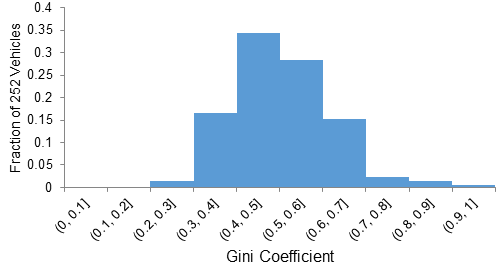
The Gini coefficient is a common measure of income inequality (Dorfman 1979), and can be used for other variables as well. In economics, the Lorenz curve illustrates the cumulative distribution of income, with percentage of individuals or households arranged in an ascending order along the x-axis (Kakwani 1977). Gini (1921) called the area between the Lorenz curve and the y = x line the “area of concentration,” and the Gini coefficient is the ratio between that area and the total area under the y = x line (or 0.5). This study calculates a Gini coefficient for each of the 252 vehicles using the 365 daily travel distance values.

Figure 2:Histogram for Gini Coefficients on 252 Vehicles’ Daily Travel

Table 2 provides summary statistics for day-to-day variability in vehicle travel per household and per vehicle. Household vehicle travel values are less variable than the per vehicle values.

The Gini coefficients of the vehicles studied have an approximately bell-shaped distribution, with 162 vehicles’ values concentrated between 0.4 and 0.6, only 2 vehicles having a Gini coefficient less than 0.35, and 8 vehicles’ coefficients being greater than 0.8. Figure 3 presents the Lorenz curves of the two extreme Gini coefficient cases in the dataset.

Figure 3:Lorenz Curves for One Year’s Worth of Daily Travel Values for Vehicles with Highest and Lowest Gini Coefficients

A regression was then run for 252 vehicles, with the Gini coefficient as the dependent variable; results are summarized in Table 3. Apart from the demographic variables, indicators for whether a vehicle’s annual travel is under 8,047 km (5,000 miles) or above 16,093 km (10,000 miles) are also used as predictors. With a total of eight independent variables, the adjusted R² equals 0.2807.

According to Table 3, the variable that has the most positive impact on the Gini coefficient is whether the annual mileage travelled by the studied vehicle falls under 8,047 km (5,000 miles). Meanwhile, the three major factors related to a lower Gini coefficient are whether the primary driver of the vehicle works full time, whether it travels more than 16,093 km (10,000 miles) a year, and whether the driver is a homemaker. Although how much the vehicle will travel is unknown, a possible approach to estimate is to ask its primary driver to select a range for vehicle travel over the past year, under the assumption that the vehicle’s travel pattern, though varying on a daily basis, tends to be constant from year to year (Oak Ridge National Laboratory 2011).

Among the drivers in the lowest quartile in Gini coefficient, more than 90% are employed full-time, significantly higher than the 75% sample average. Thirty percent are male, lower than the sample average of 46%. Their average annual vehicle travel is ~800 km (500 miles) short of the average annual travel across all the sampled drivers. When regression of annual vehicle travel is run with the same variables limited to only this quartile of drivers, an average adjusted R² of 0.374 is reached, which is higher than if run with the entire group using a full week’s data. In other words, the vehicles within the top 25% in travel homogeneity have daily vehicle travel that provides predictive power as strong as a whole week’s data from an average vehicle in the dataset for annual vehicle travel.

FINDINGS

Individuals’ travel patterns vary from day to day, so dramatic mistakes are regularly made when extrapolating one day’s vehicle travel to a full year’s. Full-week trip entries facilitated by technologies such as GPS devices improve the accuracy in annual vehicle travel prediction significantly compared to single-day and two-day trip diaries. When a daily vehicle travel value comes from a vehicle with a low (first-quartile) Gini coefficient, that vehicle’s annual vehicle travel can be better predicted than when using a full week’s data from a vehicle with an average Gini coefficient. Such consistently used vehicles are more likely to be driven by full-time employed female drivers who travel slightly less than average. However, overall higher mileage throughout the year tends to correspond to lower day-to-day variability.

ACKNOWLEDGMENTS

This work owes much credit to the NSF Sustainable Research Network research project that funded the first author’s time, and to Scott Schauer-West and Albert Coleman for editorial assistance.